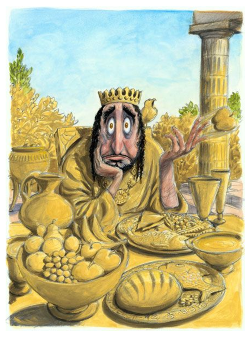
“Be careful what you wish for!” – we’ve all heard it! The story of King Midas
is there to warn us of what might happen when we’re not. Midas, a king who loves
gold, runs into a satyr and wishes that everything he touches would turn to gold.
Initially, this is fun and he walks around turning items to gold. But his
happiness is short lived. Midas realizes the downsides of his wish when he hugs
his daughter and she turns into a golden statue.
We, humans, have a notoriously difficult time specifying what we actually want,
and the AI systems we build suffer from it. With AI, this warning actually
becomes “Be careful what you reward!”. When we design and deploy an AI agent
for some application, we need to specify what we want it to do, and this
typically takes the form of a reward function: a function that tells the agent
which state and action combinations are good. A car reaching its destination is
good, and a car crashing into another car is not so good.
AI research has made a lot of progress on algorithms for generating AI behavior
that performs well according to the stated reward function, from classifiers
that correctly label images with what’s in them, to cars that are starting to
drive on their own. But, as the example of King Midas teaches us, it’s not the
stated reward function that matters: what we really need are algorithms for
generating AI behavior that performs well according to the designer or user’s
intended reward function.
Our recent work on Cooperative
Inverse Reinforcement Learning formalizes and investigates optimal
solutions to this value alignment problem — the joint problem of eliciting
and optimizing a user’s intended objective.
Subhashini Venugopalan and Lisa Anne HendricksAug 8, 2017
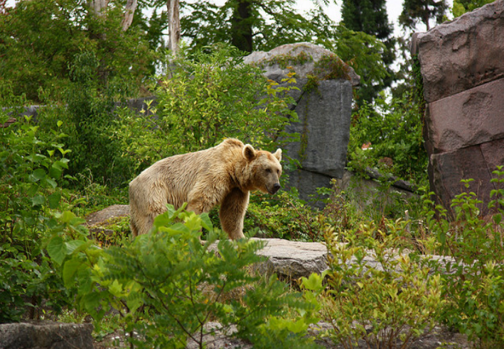
Given an image, humans can easily infer the salient entities in it, and describe the scene effectively, such as, where objects are located (in a forest or in a kitchen?), what attributes an object has (brown or white?), and, importantly, how objects interact with other objects in a scene (running in a field, or being held by a person etc.). The task of visual description aims to develop visual systems that generate contextual descriptions about objects in images. Visual description is challenging because it requires recognizing not only objects (bear), but other visual elements, such as actions (standing) and attributes (brown), and constructing a fluent sentence describing how objects, actions, and attributes are related in an image (such as the brown bear is standing on a rock in the forest).
Current State of Visual Description
LRCN [Donahue et al. ‘15]: A brown bear standing on top of a lush green field. MS CaptionBot [Tran et al. ‘16]: A large brown bear walking through a forest.
LRCN [Donahue et al. ‘15]: A black bear is standing in the grass. MS CaptionBot [Tran et al. ‘16]: A bear that is eating some grass.
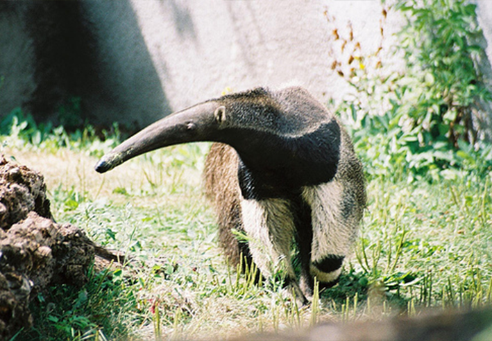
Descriptions generated by existing captioners on two images. On the left is an image of an object (bear) that is present in training data. On the right is an object (anteater) that the model hasn't seen in training.
Current visual description or image captioning models work quite well, but they can only describe objects seen in existing image captioning training datasets, and they require a large number of training examples to generate good captions. To learn how to describe an object like “jackal” or “anteater” in context, most description models require many examples of jackal or anteater images with corresponding descriptions. However, current visual description datasets, like MSCOCO, do not include descriptions about all objects. In contrast, recent works in object recognition through Convolutional Neural Networks (CNNs) can recognize hundreds of categories of objects. While object recognition models can recognize jackals and anteaters, description models cannot compose sentences to describe these animals correctly in context. In our work, we overcome this problem by building visual description systems which can describe new objects without pairs of images and sentences about these objects.
Over the last few years we have experienced an enormous data deluge, which has
played a key role in the surge of interest in AI. A partial list of some large
datasets:
ImageNet, with over 14 million images for classification and object detection.
Movielens, with 20 million user ratings of movies for collaborative filtering.
Udacity’s car dataset (at least 223GB) for training self-driving cars.
Yahoo’s 13.5 TB dataset of user-news interaction for studying human behavior.
Stochastic Gradient Descent (SGD) has been the engine fueling the
development of large-scale models for these datasets. SGD is remarkably
well-suited to large datasets: it estimates the gradient of the loss function on
a full dataset using only a fixed-sized minibatch, and updates a model many
times with each pass over the dataset.
But SGD has limitations. When we construct a model, we use a loss function
$L_\theta(x)$ with dataset $x$ and model parameters $\theta$ and attempt to
minimize the loss by gradient descent on $\theta$. This shortcut approach makes
optimization easy, but is vulnerable to a variety of problems including
over-fitting, excessively sensitive coefficient values, and possibly slow
convergence. A more robust approach is to treat the inference problem for
$\theta$ as a full-blown posterior inference, deriving a joint distribution
$p(x,\theta)$ from the loss function, and computing the posterior $p(\theta|x)$.
This is the Bayesian modeling approach, and specifically the Bayesian Neural
Network approach when applied to deep models. This recent tutorial by Zoubin
Ghahramani discusses some of the advantages of this approach.
The model posterior $p(\theta|x)$ for most problems is intractable (no closed
form). There are two methods in Machine Learning to work around intractable
posteriors: Variational Bayesian methods and Markov Chain Monte Carlo
(MCMC). In variational methods, the posterior is approximated with a simpler
distribution (e.g. a normal distribution) and its distance to the true posterior
is minimized. In MCMC methods, the posterior is approximated as a sequence of
correlated samples (points or particle densities). Variational Bayes methods
have been widely used but often introduce significant error — see this recent
comparison with Gibbs Sampling, also Figure 3 from the Variational
Autoencoder (VAE) paper. Variational methods are also more computationally
expensive than direct parameter SGD (it’s a small constant factor, but a small
constant times 1-10 days can be quite important).
MCMC methods have no such bias. You can think of MCMC particles as rather like
quantum-mechanical particles: you only observe individual instances, but they
follow an arbitrarily-complex joint distribution. By taking multiple samples you
can infer useful statistics, apply regularizing terms, etc. But MCMC methods
have one over-riding problem with respect to large datasets: other than the
important class of conjugate models which admit Gibbs sampling, there has been
no efficient way to do the Metropolis-Hastings tests required by general MCMC
methods on minibatches of data (we will define/review MH tests in a moment). In
response, researchers had to design models to make inference tractable, e.g.
Restricted Boltzmann Machines (RBMs) use a layered, undirected design to
make Gibbs sampling possible. In a recent breakthrough, VAEs use
variational methods to support more general posterior distributions in
probabilistic auto-encoders. But with VAEs, like other variational models, one
has to live with the fact that the model is a best-fit approximation, with
(usually) no quantification of how close the approximation is. Although they
typically offer better accuracy, MCMC methods have been sidelined recently in
auto-encoder applications, lacking an efficient scalable MH test.
A key aspect of intelligence is versatility – the capability of doing many
different things. Current AI systems excel at mastering a single skill, such as
Go, Jeopardy, or even helicopter aerobatics. But, when you instead ask an AI
system to do a variety of seemingly simple problems, it will struggle. A
champion Jeopardy program cannot hold a conversation, and an expert helicopter
controller for aerobatics cannot navigate in new, simple situations such as
locating, navigating to, and hovering over a fire to put it out. In contrast, a
human can act and adapt intelligently to a wide variety of new, unseen
situations. How can we enable our artificial agents to acquire such versatility?
There are several techniques being developed to solve these sorts of problems
and I’ll survey them in this post, as well as discuss a recent technique from
our lab, called model-agnostic
meta-learning. (You can check out the research paper here, and the code
for the underlying technique here.)
Current AI systems can master a complex skill from scratch, using an
understandably large amount of time and experience. But if we want our agents to
be able to acquire many skills and adapt to many environments, we cannot afford
to train each skill in each setting from scratch. Instead, we need our agents to
learn how to learn new tasks faster by reusing previous experience, rather than
considering each new task in isolation. This approach of learning to learn, or
meta-learning, is a key stepping stone towards versatile agents that can
continually learn a wide variety of tasks throughout their lifetimes.
So, what is learning to learn, and what has it been used for?
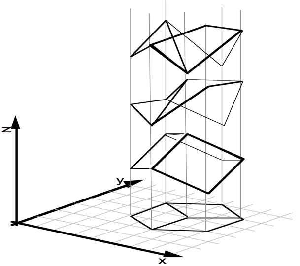
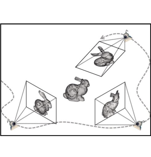
Given only a single 2D image, humans are able to effortlessly infer the rich 3D structure of the underlying scene. Since inferring 3D from 2D is an ambiguous task by itself (see e.g. the left figure below), we must rely on learning from our past visual experiences. These visual experiences solely consist of 2D projections (as received on the retina) of the 3D world. Therefore, the learning signal for our 3D perception capability likely comes from making consistent connections among different perspectives of the world that only capture partial evidence of the 3D reality. We present methods for building 3D prediction systems that can learn in a similar manner.
An image could be the projection of infinitely many 3D structures (figure from Sinha & Adelson).
Our visual experiences solely comprise of 2D projections of the 3D world.
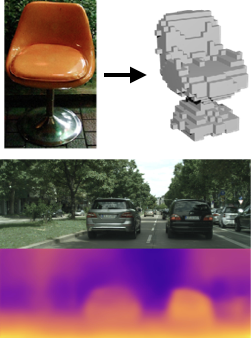
Our approach can learn from 2D projections and predict shape (top) or depth (bottom) from a single image.
Building computational models for single image 3D inference is a long-standing problem in computer vision. Early attempts, such as the Blocks World or 3D surface from line drawings, leveraged explicit reasoning over geometric cues to optimize for the 3D structure. Over the years, the incorporation of supervised learning allowed approaches to scale to more realistic settings and infer qualitative (e.g. Hoiem et al.) or quantitative (e.g. Saxena et al.) 3D representations. The trend of obtaining impressive results in realistic settings has since continued to the current CNN-based incarnations (e.g. Eigen & Fergus, Wang et al.), but at the cost of increasing reliance on direct 3D supervision, making this paradigm rather restrictive. It is costly and painstaking, if not impossible, to obtain such supervision at a large scale. Instead, akin to the human visual system, we want our computational systems to learn 3D prediction without requiring 3D supervision.
With this goal in mind, our work and several other recent approaches explore another form of supervision: multi-view observations, for learning single-view 3D. Interestingly, not only do these different works share the goal of incorporating multi-view supervision, the methodologies used also follow common principles. A unifying foundation to these approaches is the interaction between learning and geometry, where predictions made by the learning system are encouraged to be ‘geometrically consistent’ with the multi-view observations. Therefore, geometry acts as a bridge between the learning system and the multi-view training data.
We recently developed a principled way to incorporate safety requirements and other constraints directly into a family of state-of-the-art deep RL algorithms. Our approach, Constrained Policy Optimization (CPO), makes sure that the agent satisfies constraints at every step of the learning process. Specifically, we try to satisfy constraints on costs: the designer assigns a cost and a limit for each outcome that the agent should avoid, and the agent learns to keep all of its costs below their limits.
This kind of constrained RL approach has been around for a long time, and has even inspired closely-related work here at Berkeley on probabilistically safe policy transfer. But CPO is the first algorithm that makes it practical to apply deep RL to the constrained setting for general situations—and furthermore, it comes with theoretical performance guarantees.
In our paper, we describe an efficient way to run CPO, and we show that CPO can successfully train neural network agents to maximize reward while satisfying constraints in tasks with realistic robot simulations. If you want to try applying CPO to your constrained RL problem, we’ve open-sourced our code.
Reliable robot grasping across many objects is challenging due to sensor noise
and occlusions that lead to uncertainty about the precise shape, position, and
mass of objects. The Dexterity Network (Dex-Net) 2.0 is a project centered on
using physics-based models of robust robot grasping to generate massive datasets
of parallel-jaw grasps across thousands of 3D CAD object models. These datasets
are used to train deep neural networks to plan grasps from a point clouds on a
physical robot that can lift and transport a wide variety of objects.
To facilitate reproducibility and future research, this blog post announces the
release of the:
Dexterity Network (Dex-Net) 2.0 dataset: 6.7 million pairs of synthetic point clouds and grasps with robustness labels. [link to data folder]
Grasp Quality CNN (GQ-CNN) model: 18 million parameters trained on the Dex-Net 2.0 dataset. [link to our models]
GQ-CNN Python Package: Code to replicate our GQ-CNN training results on synthetic data (note System Requirements below). [link to code].
In the post, we also summarize the methods behind Dex-Net 2.0 (1), our
experimental results on a real robot, and details on the datasets, models, and
code.
(Joint work with Ronghang Hu, Marcus Rohrbach, Trevor Darrell, Dan Klein and
Kate Saenko.)
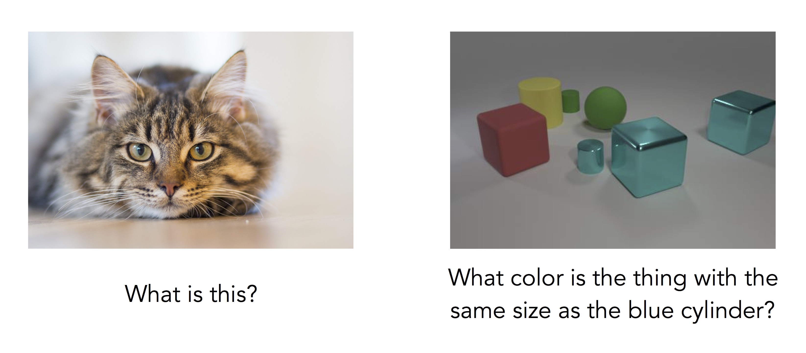
Suppose we’re building a household robot, and want it to be able to answer
questions about its surroundings. We might ask questions like these:
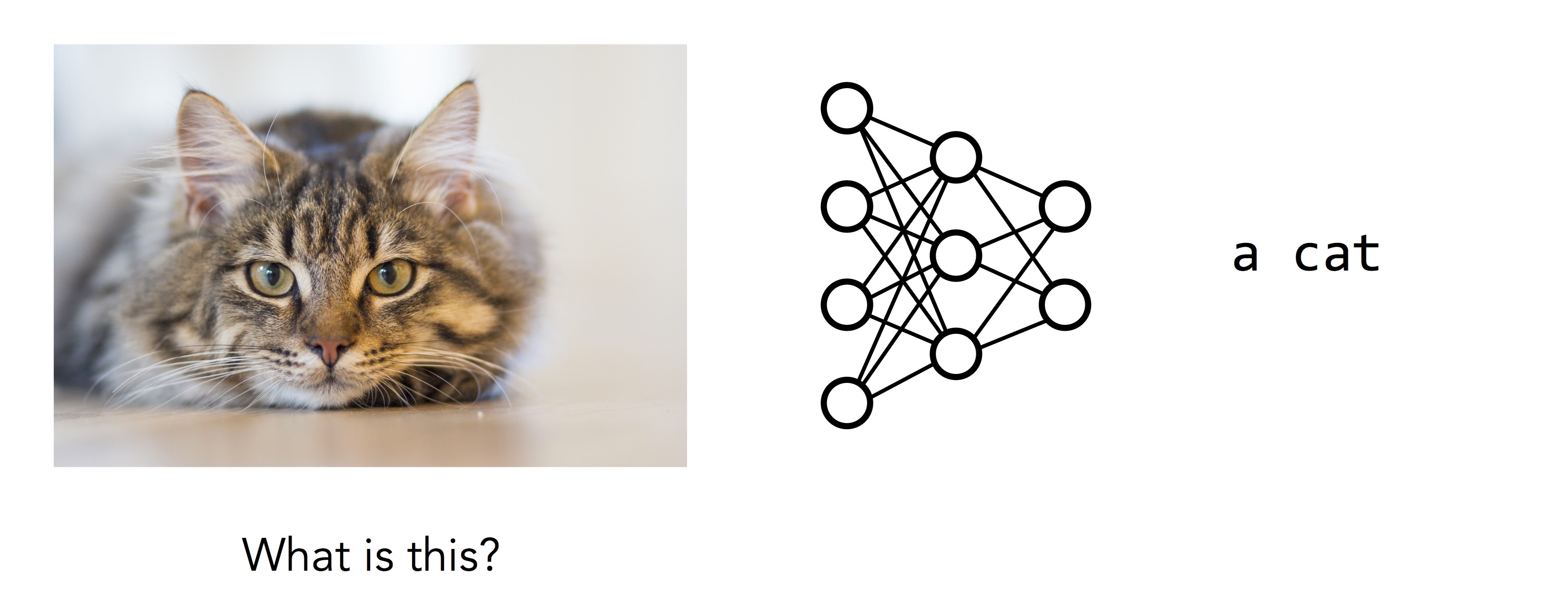
How can we ensure that the robot can answer these questions correctly? The
standard approach in deep learning is to collect a large dataset of questions,
images, and answers, and train a single neural network to map directly from
questions and images to answers. If most questions look like the one on the
left, we have a familiar image recognition problem, and these kinds of
monolithic approaches are quite effective:
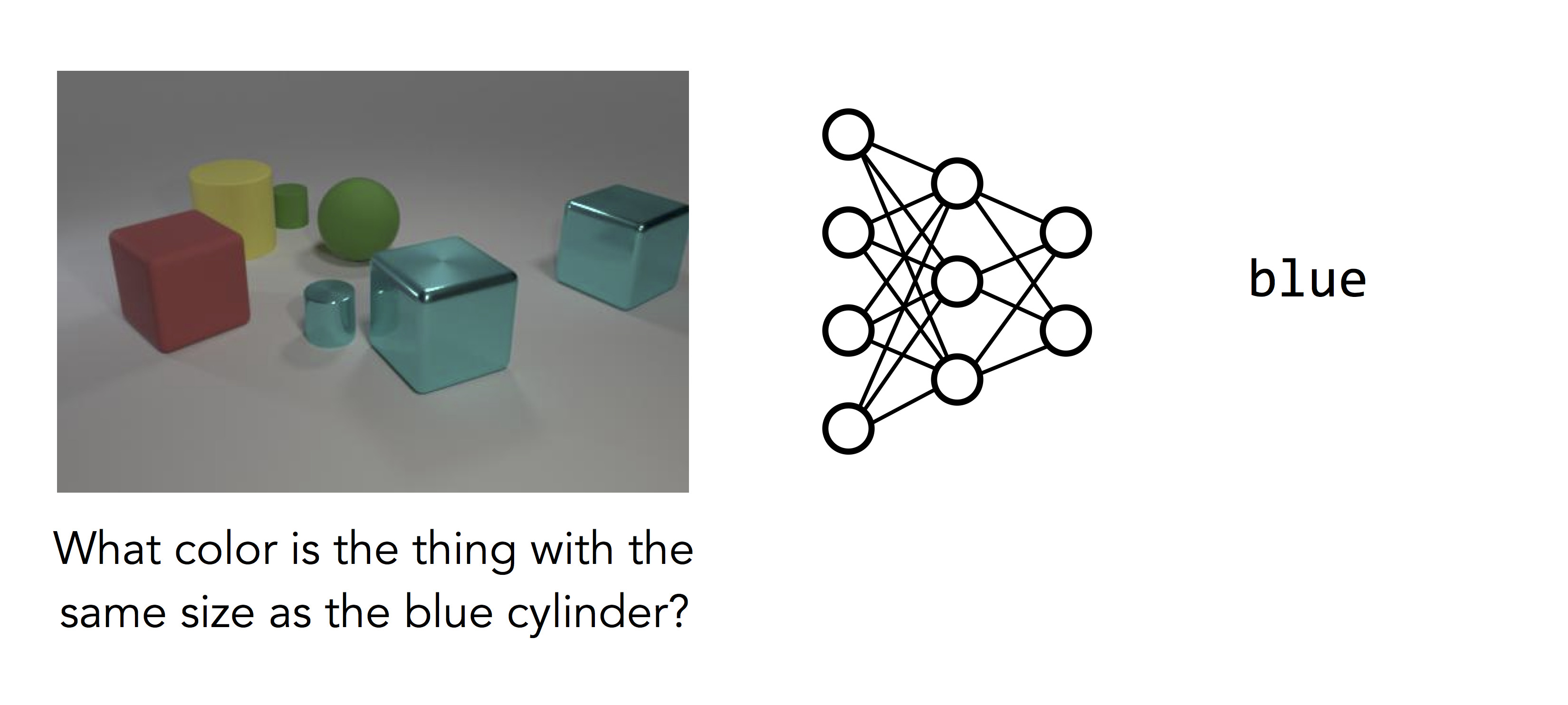
But things don’t work quite so well for questions like the one on the
right:
Here the network we trained has given up and guessed the most common color in
the image. What makes this question so much harder? Even though the image is
cleaner, the question requires many steps of reasoning: rather than
simply recognizing the main object in the image, the model must first find the
blue cylinder, locate the other object with the same size, and then determine
its color. This is a complicated computation, and it’s a computation
specific to the question that was asked. Different questions require
different sequences of steps to solve.
The dominant paradigm in deep learning is a "one size fits all" approach: for
whatever problem we’re trying to solve, we write down a fixed model architecture
that we hope can capture everything about the relationship between the input and
output, and learn parameters for that fixed model from labeled training
data.
But real-world reasoning doesn’t work this way: it involves a variety of
different capabilities, combined and synthesized in new ways for every new
challenge we encounter in the wild. What we need is a model that can
dynamically determine how to reason about the problem in front of it—a
network that can choose its own structure on the fly. In this post, we’ll talk
about a new class of models we call neural module networks
(NMNs), which incorporate this more flexible approach to problem-solving while
preserving the expressive power that makes deep learning so effective.
Berkeley AI Research (BAIR) brings together researchers at UC Berkeley across
the areas of computer vision, machine learning, natural language processing,
planning, and robotics, and each year we publish cutting edge research across
all of these areas. Dissemination of scientific results is a core component of
our mission, and while the traditional avenues for fulfilling this mission –
publications and presentations at academic conferences – continue to be the
primary method for disseminating our results, we must also strive to make our
results accessible, easily interpretable, and available to all. As part of this
effort, we are launching the BAIR Blog, a general audience blog where we will
present and discuss recent results in computer vision, deep learning, robotics,
NLP, and a variety of other areas where BAIR conducts cutting-edge research. Our
aim with the BAIR Blog will be to present recent scientific findings in a format
that is engaging, accessible, but at the same time informative for readers with
all levels of expertise. Our inaugural post describes some recent work at BAIR
at the intersection of vision and natural language processing. Posts on a
variety of other topics will follow on a weekly basis.