
Fig 1. A wavelet adapting to new data.
Recent deep neural networks (DNNs) often predict extremely well, but sacrifice interpretability and computational efficiency. Interpretability is crucial in many disciplines, such as science and medicine, where models must be carefully vetted or where interpretation is the goal itself. Moreover, interpretable models are concise and often yield computational efficiency.
In our recent paper, we propose adaptive wavelet distillation (AWD), a method which distills information from a trained DNN into a wavelet transform. Surprisingly, we find that the resulting transform improves state-of-the-art predictive performance, despite being extremely concise, interpretable, and computationally efficient! (The trick is making wavelets adaptive and using interpretations, more on that later). In close collaboration with domain experts, we show how AWD addresses challenges in two real-world settings: cosmological parameter inference🌌 and molecular-partner prediction🦠.
Background and motivation
What’s a wavelet? Wavelets are an extremely powerful signal-processing tool for transforming structured signals, such as images and time-series data. Wavelets have many useful properties, including fast computation, multi-scale structure, an orthonormal basis, and interpretation in both spatial and frequency domains (if you’re interested, see this whole book on wavelets). This makes wavelets a great candidate for an interpretable model in many signal-processing applications. Traditionally, wavelets are hand-designed to satisfy human-specified criteria. Here, we allow wavelets to be adaptive: they change their form based on the given input data and trained DNN.
TRIM In order to adapt the wavelet model based on a given DNN, we need a way to convey information from the DNN to the wavelet parameters. This can be done using Transformation Importance (TRIM). Given a transformation $\Psi$ (here the wavelet transform) and an input $x$, TRIM obtains feature importances for a given DNN $f$ in the transformed domain using a simple reparameterization trick: the DNN is pre-prended with the transform $\Psi$, coefficients $\Psi x$ are extracted, and then the inverse transform is re-applied before being fed into the network $f(\Psi^{-1} \Psi x$). This allows for computing the interpretations $TRIM_f(\Psi x_i)$ using any popular method, such as SHAP, ACD, IG, or the gradient of the prediction with respect to the wavelet coefficients (that’s what we use here - it’s simple and seems to work).
Adaptive wavelet distillation: some quick intuition and math
We’re now ready to define AWD. We want our learned wavelet model to satisfy three properties: (i) represent our data well, (ii) be a valid wavelet, and (iii) distill information from a trained DNN. Each of the losses in the equation below corresponds to these three properies (for full details see eq. 8 in the paper). $x_i$ represents the $i$-th input example, $wave$ represents the wavelet parameters, and $\Psi x_i$ denotes the wavelet coefficients of $x_i$. $\lambda$ is a hyperparameter penalizing the sparsity of the wavelet coefficients, and $\gamma$ is a hyperparameter controlling the strength of the interpretation loss.
\[\begin{align}\underset{wave}{\text { minimize }}\mathcal L (wave)&= \underbrace{\frac{1}{m}\sum_{i} ||x_i - \Psi^{-1} \Psi x_i||_{2}^{2}}_{\text {(i) Reconstruction loss }} +\underbrace{\frac{1}{m}\sum_i W(wave, x_i; \lambda)}_{\text {(ii) Wavelet loss }} \\&+\underbrace{\gamma \sum_{i} ||TRIM_f(\Psi x_i)||_1}_{\text {(iii) Interpretation loss }}\end{align}\]The reconstruction loss (i) ensures that the wavelet transform is invertible, thus preserving all the information in the input data. The wavelet loss (ii) ensures that the learned filters yield a valid wavelet transform, and also that the wavelets provide a sparse representation of the input, thus providing compression.
Finally, the interpretation loss (iii) is a key difference between AWD and existing adaptive wavelet techniques. It incorporates information about the DNN and the outcome by forcing the wavelet representation to concisely explain the DNN’s predictions at different scales and locations.
🌌 Estimating a fundamental parameter surrounding the origin of the universe
Now, for the fun stuff. We turn to a cosmology problem, where AWD helps replace DNNs with a more interpretable alternative.
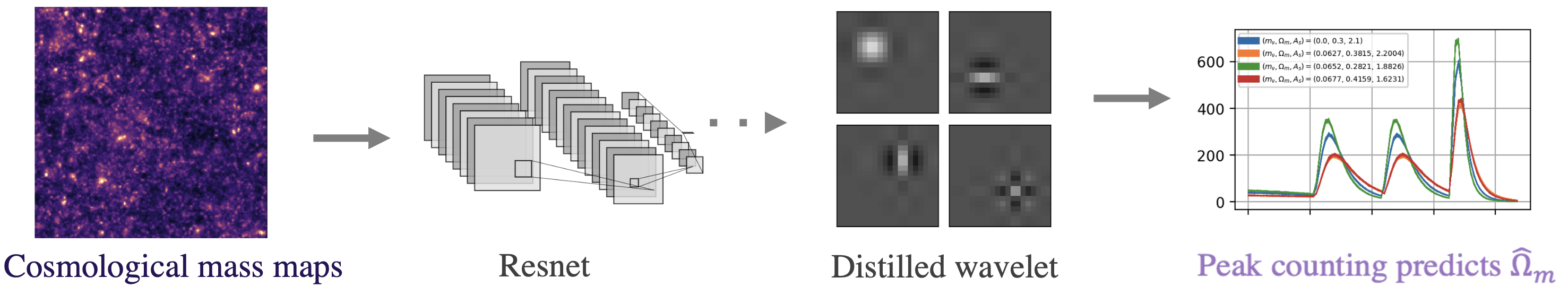
Fig 2. Pipeline for cosmological parameter prediction.
Specifically, we consider maps of the mass distribution in the universe, which come from sophisticated cosmological simulations. These maps contain a wealth of physical information of interest, such as the total matter density in the universe, $\Omega_m$. Given a large amount of these maps, we aim to predict the values of fundamental cosmological parameters such as $\Omega_m$.
Traditionally, these parameters are predicted using interpretable methods, such as analyzing the maps’ power spectrum, but recent works have suggested DNNs can better predict these cosmological parameters. Here, we aim to use the predictive power of DNNs while also maintaining interpretability by distilling a DNN into a predictive AWD model. In this context, it is critically important to obtain interpretability, as it provides deeper scientific understanding in how parameters such as $\Omega_m$ manifest in mass maps, can help design optimal experiments, and identify numerical artifacts in simulations
As shown in Fig 2, we first fit a DNN and then distill a wavelet from the trained model, which we use to make predictions following a simple peak-counting scheme. Table 1 below shows the results. They are surprisingly good for how simple the model is! Our AWD model ends up with only 9 fitted parameters but lowers the prediction error over all baseline methods, including the original DNN (the Roberts-cross and Laplace filter baselines are from this very cool state-of-the-art nature paper).
| AWD | Roberts-Cross | Laplace | DB5 Wavelet | Resnet | |
|---|---|---|---|---|---|
| Regression (RMSE) | 1.029 | 1.259 | 1.369 | 1.569 | 1.156 |
Table 1. Prediction and compression performance for AWD outperforms baselines.
Besides predictive performance, the AWD model is extremely interpretable; it matches the form of model previously used in cosmology and the symmetric nature of the distilled wavelet matches prior knowledge regarding $\Omega_m$. It is also extremely fast and efficient to run inference and provides a compressed representation of our data.
🦠 Molecular partner-prediction for a central process in cell biology
We now turn our attention to a crucial question in cell biology related to the internalization of macromolecules via clathrin-mediated endocytosis (CME). CME is the primary pathway for entry into the cell, making it essential to eukaryotic life. Crucial to understanding CME is the ability to readily distinguish whether or not the recruitment of certain molecules will allow for endocytosis, i.e., successfully transporting an object into a cell.
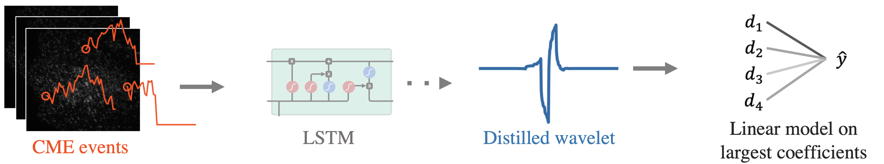
Fig 3. Pipeline for CME prediction using AWD.
Here, we aim to identify successful CME events from cell videos. We use a recently published dataset which tags two molecules: clathrin, which is used as the predictor variable since it usually precedes an event, and auxilin, which is used as the target variable since it signals whether endocytostis succesfully occurs (see data details in the paper). Time-series are extracted from cell videos and fed to a DNN to predict the auxilin outcome. The DNN predicts well, but has extremely poor interpretability and computational cost, so we distill it into a wavelet model through AWD.
As shown in Fig 3, we distill a single wavelet from the trained DNN, and then make predictions using a linear model on the largest wavelet coefficients at each scale. Table 2 shows the prediction results: AWD outperforms the standard wavelet and also the original LSTM model (which we spent years building)! What’s more, the model compressed the input, was way smaller (it has only 10 parameters 🤏), and is extremely efficient to run.
| AWD | Standard Wavelet (DB5) | LSTM | |
|---|---|---|---|
| Regression ($R^2$ score) | 0.262 | 0.197 | 0.237 |
Table 2. Prediction and compression performance for AWD outperforms baselines.
Conclusion
The results here show the impressive power of a simple linear transform when it is adapted in the right manner. Using AWD, we were able to distill information contained in large DNNs into a wavelet model, which is smaller, faster, and much more interpretable. There’s a lot left to do at the intersection of wavelets, neural nets, and interpretability. Check out our adaptive wavelets package if you’re interested in using adaptive wavelets or extending them to new settings.
This post is based on the paper “Adaptive wavelet distillation from neural networks through interpretations”, to be presented at NeurIPS 2021. This is joint work with amazing scientific collaborators Francois Lanusse and Gokul Upadhyayula. We provide a python package to run the method on new data and reproduce our results.