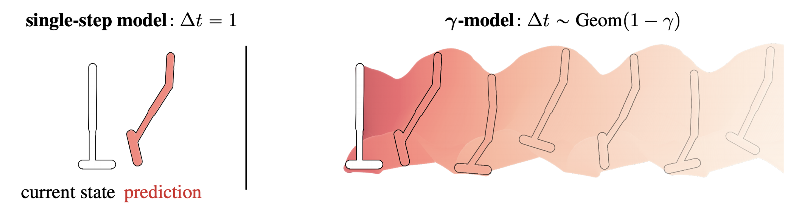
Standard single-step models have a horizon of one. This post describes a method for training predictive dynamics models in continuous state spaces with an infinite, probabilistic horizon.
Reinforcement learning algorithms are frequently categorized by whether they predict future states at any point in their decision-making process. Those that do are called model-based, and those that do not are dubbed model-free. This classification is so common that we mostly take it for granted these days; I am guilty of using it myself. However, this distinction is not as clear-cut as it may initially seem.
In this post, I will talk about an alternative view that emphases the mechanism of prediction instead of the content of prediction. This shift in focus brings into relief a space between model-based and model-free methods that contains exciting directions for reinforcement learning. The first half of this post describes some of the classic tools in this space, including generalized value functions and the successor representation. The latter half is based on our recent paper about infinite-horizon predictive models, for which code is available here.
The what versus how of prediction
The dichotomy between model-based and model-free algorithms focuses on what is predicted directly: states or values. Instead, I want to focus on how these predictions are made, and specifically how these approaches deal with the complexities arising from long horizons.
Dynamics models, for instance, approximate a single-step transition distribution, meaning that they are trained on a prediction problem with a horizon of one. In order to make a short-horizon model useful for long-horizon queries, its single-step predictions are composed in the form of sequential model-based rollouts. We could say that the “testing” horizon of a model-based method is that of the rollout.
In contrast, value functions themselves are long-horizon predictors; they need not be used in the context of rollouts because they already contain information about the extended future. In order to amortize this long-horizon prediction, value functions are trained with either Monte Carlo estimates of expected cumulative reward or with dynamic programming. The important distinction is now that the long-horizon nature of the prediction task is dealt with during training instead of during testing.
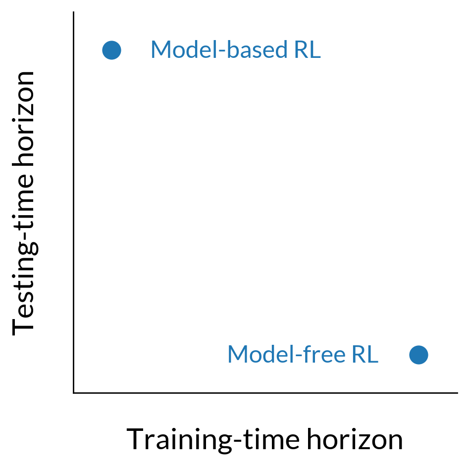
We can organize reinforcement learning algorithms in terms of when they deal with long-horizon complexity. Dynamics models train for a short-horizon prediction task but are deployed using long-horizon rollouts. In contrast, value functions amortize the work of long-horizon prediction at training, so a single-step prediction (and informally, a shorter "horizon") is sufficient during testing.
Taking this view, the fact that models predict states and value functions predict cumulative rewards is almost a detail. What really matters is that models predict immediate next states and value functions predict long-term sums of rewards. This idea is nicely summarized in a line of work on generalized value functions, describing how temporal difference learning may be used to make long-horizon predictions about any kind of cumulant, of which a reward function is simply one example.
This framing also suggests that some phenomena we currently think of as distinct, like compounding model prediction errors and bootstrap error accumulation, might actually be different lenses on the same problem. The former describes the growth in error over the course of a model-based rollout, and the latter describes the propagation of error via the Bellman backup in model-free reinforcement learning. If models and value functions differ primarily in when they deal with horizon-based difficulties, then it should come as no surprise that the testing-time error compounding of models has a direct training-time analogue in value functions.
A final reason to be interested in this alternative categorization is that it allows us to think about hybrids that do not make sense under the standard dichotomy. For example, if a model were to make long-horizon state predictions by virtue of training-time amortization, it would avoid the need for sequential model-based rollouts and circumvent testing-time compounding errors. The remaining sections describe how we can build such a model, beginning with the foundation of the successor representation and then introducing new work for making this form of prediction compatible with continuous spaces and neural samplers.
The successor representation
The successor representation (SR), an idea influential in both cognitive science and machine learning, is a long-horizon, policy-dependent dynamics model. It leverages the insight that the same type of recurrence relation used to train \(Q\)-functions: \[ Q(\mathbf{s}_t, \mathbf{a}_t) \leftarrow \mathbb{E}_{\mathbf{s}_{t+1}} [r(\mathbf{s}_{t}, \mathbf{a}_t, \mathbf{s}_{t+1}) + \gamma V(\mathbf{s}_{t+1})] \] may also be used to train a model that predicts states instead of values: \[ M(\mathbf{s}_{t}, \mathbf{a}_t) \leftarrow \mathbb{E}_{\mathbf{s}_{t+1}} [\mathbf{1}(\mathbf{s}_{t+1}) + \gamma M(\mathbf{s}_{t+1})] \tag*{(1)} \]
The key difference between the two is that the scalar rewards \(r(\mathbf{s}_t, \mathbf{a}_t, \mathbf{s}_{t+1})\) from the \(Q\)-function recurrence are now replaced with one-hot indicator vectors \(\mathbf{1}(\mathbf{s}_{t+1})\) denoting states. As such, SR training may be thought of as vector-valued \(Q\)-learning. The size of the “reward” vector, as well as the successor predictions \(M(\mathbf{s}_t, \mathbf{a}_t)\) and \(M(\mathbf{s}_t)\), is equal to the number of states in the MDP.
In contrast to standard dynamics models, which approximate a single-step transition distribution, SR approximates what is known as the discounted occupancy: \[ \mu(\mathbf{s}_e \mid \mathbf{s}_t, \mathbf{s}_t) = (1 - \gamma) \sum_{\Delta t=1}^{\infty} \gamma^{\Delta t - 1} p( \mathbf{s}_{t+\Delta t} = \mathbf{s}_e \mid \mathbf{s}_t, \mathbf{a}_t, \pi ) \]
This occupancy is a weighted mixture over an infinite series of multi-step models, with the mixture weights being controlled by a discount factor \(\gamma\).1 2 Setting \(\gamma=0\) recovers a standard single-step model, and any \(\gamma \in (0,1)\) induces a model with an infinite, probabilistic horizon. The predictive lookahead of the model qualitatively increases with larger \(\gamma\).
The successor representation of a(n optimal) rat in a maze3, showing the rat’s path with a probabilistic horizon determined by discount factor \(\gamma\).
Generative models in continuous spaces: from SR to \(\boldsymbol{\gamma}\)-models
Continuous adaptations of SR replace the one-hot state indicator \(\mathbf{1}(\mathbf{s}_t)\) in Equation 1 with a learned state featurization \(\phi(\mathbf{s}_t, \mathbf{a}_t)\), giving a recurrence of the form: \[ \psi(\mathbf{s}_t, \mathbf{a}_t) \leftarrow \phi(\mathbf{s}_t, \mathbf{a}_t) + \gamma \mathbb{E}_{\mathbf{s}_{t+1}} [\psi(\mathbf{s}_{t+1})] \]
This is not a generative model in the usual sense, but is instead known as an expectation model: \(\psi\) denotes the expected feature vector \(\phi\). The advantage to this approach is that an expectation model is easier to train than a generative model. Moreover, if rewards are linear in the features, an expectation model is sufficient for value estimation.
However, the limitation of an expectation model is that it cannot be employed in some of the most common use-cases of predictive dynamics models. Because \(\psi(\mathbf{s}_t, \mathbf{a}_t)\) only predicts a first moment, we cannot use it to sample future states or perform model-based rollouts.
To overcome this limitation, we can turn the discriminative update used in SR and its continuous variants into one suitable for training a generative model \({\color{#D62728}\mu}\): \[ \max_{\color{#D62728}\mu} \mathbb{E}_{\mathbf{s}_t, \mathbf{a}_t, \mathbf{s}_{t+1} \sim \mathcal{D}} [ \mathbb{E}_{ \mathbf{s}_e \sim (1-\gamma) p(\cdot \mid \mathbf{s}_t, \mathbf{a}_t) + \gamma {\color{#D62728}\mu}(\cdot \mid \mathbf{s}_{t+1}) } [\log {\color{#D62728}\mu}(\mathbf{s}_e \mid \mathbf{s}_t, \mathbf{a}_t)] ] \]
At first glance, this looks like a standard maximum likelihood objective. The important difference is that the distribution over which the inner expectation is evaluated depends on the model \({\color{#D62728}\mu}\) itself. Instead of a bootstrapped target value like those commonly used in model-free algorithms, we now have a bootstrapped target distribution. \[ \underset{ \vphantom{\Huge\Sigma} \Large \text{target value} }{ r + \gamma V } ~~~~~~~~ \Longleftrightarrow ~~~~~~~~ \underset{ \vphantom{\Huge\Sigma} \Large \text{target }\color{#D62728}{\text{distribution}} }{ (1-\gamma) p + \gamma {\color{#D62728}\mu} } \] Varying the discount factor \(\gamma\) in the target distribution yields models that predict increasingly far into the future.
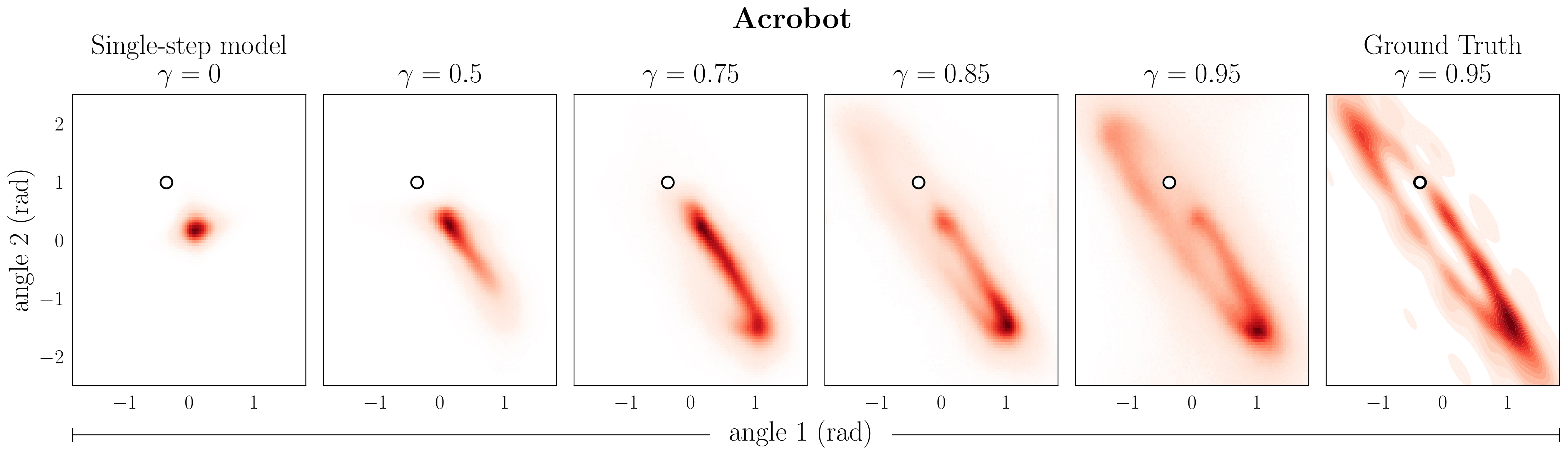
Predictions of a \(\gamma\)-model for varying discounts \(\gamma\). The rightmost column shows Monte Carlo estimates of the discounted occupancy corresponding to \(\gamma=0.95\) for reference. The conditioning state is denoted by \(\circ\).
In the spirit of infinite-horizon model-free control, we refer to this formulation as infinite-horizon prediction and the corresponding model as a \(\gamma\)-model. Because the bootstrapped maximum likelihood objective circumvents the need for reward vectors the size of the state space, \(\gamma\)-model training is suitable for continuous spaces while retaining an interpretation as a generative model. In our paper we show how to instantiate \(\gamma\)-models as both normalizing flows and generative adversarial networks.
Generalizing model-based control with \(\boldsymbol{\gamma}\)-models
Replacing single-step dynamics models with \(\gamma\)-models leads to generalizations of some of the staples of model-based control:
Rollouts: \(\gamma\)-models divorce timestep from model step. As opposed to incrementing one timestep into the future with every prediction, \(\gamma\)-model rollout steps have a negative binomial distribution over time. It is possible to reweight these \(\gamma\)-model steps to simulate the predictions of a model trained with higher discount.
Whereas conventional dynamics models predict a single step into the future, \(\gamma\)-model rollout steps have a negative binomial distribution over time. The first step of a \(\gamma\)-model has a geometric distribution from the special case of \(~\text{NegBinom}(1, p) = \text{Geom}(1-p)\).
Value estimation: Single-step models estimate values using long model-based rollouts, often between tens and hundreds of steps long. In contrast, values are expectations over a single feedforward pass of a \(\gamma\)-model. This is similar to a decomposition of value as an inner product, as seen in successor features and deep SR. In tabular spaces with indicator rewards, the inner product and expectation are the same!
Because values are expectations of reward over a single step of a \(\gamma\)-model, we can perform value estimation without sequential model-based rollouts.
Terminal value functions: To account for truncation error in single-step model-based rollouts, it is common to augment the rollout with a terminal value function. This strategy, sometimes referred to as model-based value expansion (MVE), has an abrupt handoff between the model-based rollout and the model-free value function. We can derive an analogous strategy with a \(\gamma\)-model, called \(\gamma\)-MVE, that features a gradual transition between model-based and model-free value estimation. This value estimation strategy can be incorporated into a model-based reinforcement learning algorithm for improved sample-efficiency.
\(\gamma\)-MVE features a gradual transition between model-based and model-free value estimation.
This post is based on the following paper:
-
\(\gamma\)-Models: Generative Temporal Difference Learning for Infinite-Horizon Prediction
Michael Janner, Igor Mordatch, and Sergey Levine
Neural Information Processing Systems (NeurIPS), 2020.
Open-source code (runs in your browser!)
-
The \(e\) subscript in \(\mathbf{s}_e\) is short for "exit", which comes from an interpretation of the discounted occupancy as the exit state in a modified MDP in which there is a constant \(1-\gamma\) probability of termination at each timestep.↩
-
Because the discounted occupancy plays such a central role in reinforcement learning, its approximation by Bellman equations has been a focus in multiple lines of research. For example, option models and \(\beta\)-models describe generalizations of this idea that allow for state-dependent termination conditions and arbitrary timestep mixtures.↩
-
If this particular maze looks familiar, you might have seen it in Tolman’s Cognitive Maps in Rats and Men. (Our web version has been stretched slightly horizontally.)↩
References