An earlier version of this post is on the RISELab blog. It is posted here with the permission of the authors.

We just rolled out general support for multi-agent reinforcement learning in Ray RLlib 0.6.0. This blog post is a brief tutorial on multi-agent RL and how we designed for it in RLlib. Our goal is to enable multi-agent RL across a range of use cases, from leveraging existing single-agent algorithms to training with custom algorithms at large scale.

Why multi-agent reinforcement learning?

We’ve observed that in applied RL settings, the question of whether it makes sense to use multi-agent algorithms often comes up. Compared to training a single policy that issues all actions in the environment, multi-agent approaches can offer:

A more natural decomposition of the problem. For example, suppose one wants to train policies for cellular antenna tilt control in urban environments. Instead of training a single “super-agent” that controls all the cellular antennas in a city, it is more natural to model each antenna as a separate agent in the environment because only neighboring antennas and user observations are relevant to each site. In general, we may wish to have each agent’s action and/or observation space restricted to only model the components that it can affect and those that affect it.
Potential for more scalable learning. First, decomposing the actions and observations of a single monolithic agent into multiple simpler agents not only reduces the dimensionality of agent inputs and outputs, but also effectively increases the amount of training data generated per step of the environment.

Second, partitioning the action and observation spaces per agent can play a similar role to the approach of imposing temporal abstractions, which has been successful in increasing learning efficiency in the single-agent setting. Relatedly, some of these hierarchical approaches can be implemented explicitly as multi-agent systems.

Finally, good decompositions can also lead to the learning of policies that are more transferable across different variations of an environment, i.e., in contrast to a single super-agent that may over-fit to a particular environment.

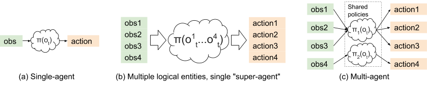
Figure 1: Single-agent approaches (a) and (b) in comparison with multi-agent RL (c).

Some examples of multi-agent applications include:

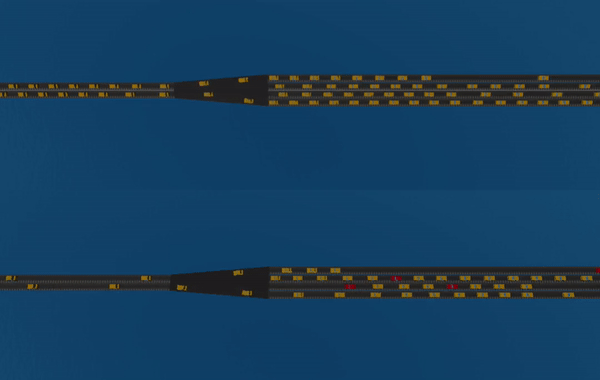
Traffic congestion reduction: It turns out that by intelligently controlling the speed of a few autonomous vehicles we can drastically increase the traffic flow. Multi-agent can be a requirement here, since in mixed-autonomy settings, it is unrealistic to model traffic lights and vehicles as a single agent, which would involve the synchronization of observations and actions across all agents in a wide area.

Flow simulation, without AVs and then with AV agents (red vehicles):

Antenna tilt control: The joint configuration of cellular base stations can be optimized according to the distribution of usage and topology of the local environment. Each base station can be modeled as one of multiple agents covering a city.

OpenAI Five: Dota 2 AI agents are trained to coordinate with each other to compete against humans. Each of the five AI players is implemented as a separate neural network policy and trained together with large-scale PPO.

Introducing multi-agent support in RLlib

In this blog post we introduce general purpose support for multi-agent RL in RLlib, including compatibility with most of RLlib’s distributed algorithms: A2C / A3C, PPO, IMPALA, DQN, DDPG, and Ape-X. In the remainder of this blog post we discuss the challenges of multi-agent RL, show how to train multi-agent policies with these existing algorithms, and also how to implement specialized algorithms that can deal with the non-stationarity and increased variance of multi-agent environments.

There are currently few libraries for multi-agent RL, which increases the initial overhead of experimenting with multi-agent approaches. Our goal is to reduce this friction and make it easy to go from single-agent to multi-agent RL in both research and application.

Why supporting multi-agent is hard

Building software for a rapidly developing field such as RL is challenging, multi-agent especially so. This is in part due to the breadth of techniques used to deal with the core issues that arise in multi-agent learning.

Consider one such issue: environment non-stationarity. In the below figure, the red agent’s goal is to learn how to regulate the speed of the traffic. The blue agents are also learning, but only to greedily minimize their own travel time. The red agent may initially achieve its goal by simply driving at the desired speed. However, in a multi-agent environment, the other agents will learn over time to meet their own goals – in this case, bypassing the red agent. This is problematic since from a single-agent view (i.e., that of the red agent), the blue agents are “part of the environment”. The fact that environment dynamics are changing from the perspective of a single agent violates the Markov assumptions required for the convergence of Q-learning algorithms such as DQN.

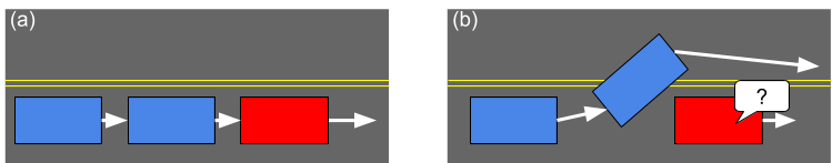
Figure 2: Non-stationarity of environment: Initially (a), the red agent learns to regulate the speed of the traffic by slowing down. However, over time the blue agents learn to bypass the red agent (b), rendering the previous experiences of the red agent invalid.

A number of algorithms have been proposed that help address this issue, e.g., LOLA, RIAL, and Q-MIX. At a high level, these algorithms take into account the actions of the other agents during RL training, usually by being partially centralized for training, but decentralized during execution. Implementation wise, this means that the policy networks may have dependencies on each other, i.e., through a mixing network in Q-MIX:

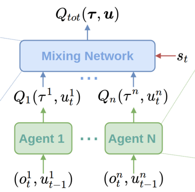
Figure 3: The Q-mix network architecture, from QMIX: Monotonic Value Function Factorisation for Deep Multi-Agent Reinforcement Learning. Individual Q-estimates are aggregated by a monotonic mixing network for efficiency of final action computation.

Similarly, policy-gradient algorithms like A3C and PPO may struggle in multi-agent settings, as the credit assignment problem becomes increasingly harder with more agents. Consider a traffic gridlock between many autonomous agents. It is easy to see that the reward given to an agent – here reflecting that traffic speed has dropped to zero – will have less and less correlation with the agent’s actions as the number of agents increases:

Figure 4: High variance of advantage estimates: In this traffic gridlock situation, it is unclear which agents' actions contributed most to the problem -- and when the gridlock is resolved, from any global reward it will be unclear which agents get credit.

One class of approaches here is to model the effect of other agents on the environment with centralized value functions (the “Q” boxes in Figure 5) function, as done in MA-DDPG. Intuitively, the variability of individual agent advantage estimates can be greatly reduced by taking into account the actions of other agents:

Figure 5: The MA-DDPG architecture, from Multi-Agent Actor-Critic for Mixed Cooperative-Competitive Environments. Policies run using only local information at execution time, but may take advantage of global information at training time.

So far we’ve seen two different challenges and approaches for tackling multi-agent RL. That said, in many settings training multi-agent policies using single-agent RL algorithms can yield surprisingly strong results. For example, OpenAI Five has been successful using only a combination of large-scale PPO and a specialized network model. The only considerations for multi-agent are the annealing of a “team spirit” hyperparameter that influences the level of shared reward, and a shared “max-pool across Players” operation in the model to share observational information.

Multi-agent training in RLlib

So how can we handle both these specialized algorithms and also the standard single-agent RL algorithms in multi-agent settings? Fortunately RLlib’s design makes this fairly simple. The relevant principles to multi-agent are as follows:

Policies are represented as objects: All gradient-based algorithms in RLlib declare a policy graph object, which includes a policy model $\pi_\theta(o_t)$, a trajectory postprocessing function $post_\theta(traj)$, and finally a policy loss $L(\theta; X)$. This policy graph object specifies enough for the distributed framework to execute environment rollouts (by querying $\pi_\theta$), collate experiences (by applying $post_\theta$), and finally to improve the policy (by descending $L(\theta; X)$).
Policy objects are black boxes: To support multi-agent, RLlib just needs to manage the creation and execution of multiple policy graphs per environment, and add together the losses during policy optimization. Policy graph objects are treated largely as black boxes by RLlib, which means that they can be implemented in any framework including TensorFlow and PyTorch. Moreover, policy graphs can internally share variables and layers to implement specialized algorithms such as Q-MIX and MA-DDPG, without special framework support.

To make the application of these principles concrete, In the next few sections we walk through code examples of using RLlib’s multi-agent APIs to execute multi-agent training at scale.

Multi-agent environment model

We are not aware of a standard multi-agent environment interface, so we wrote our own as a straightforward extension of the gym interface. In a multi-agent environment, there can be multiple acting entities per step. As a motivating example, consider a traffic control scenario (Figure 6) where multiple controllable entities (e.g., traffic lights, autonomous vehicles) work together to reduce highway congestion.

In this scenario,

Each of these agents can act at different time-scales (i.e., act asynchronously).
Agents can come and go from the environment as time progresses.

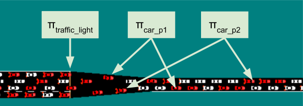
Figure 6. RLlib multi-agent environments can model multiple independent agents that come and go over time. Different policies can be assigned to agents as they appear.

This is formalized in the MultiAgentEnv interface, which can returns observations and rewards from multiple ready agents per step:

# Example: using a multi-agent env
> env = MultiAgentTrafficEnv(num_cars=20, num_traffic_lights=5)

# Observations are a dict mapping agent names to their obs. Not all
# agents need to be present in the dict in each time step.
> print(env.reset())
{
    "car_1": [[...]],
    "car_2": [[...]],
    "traffic_light_1": [[...]],
}

# Actions should be provided for each agent that returned an observation.
> new_obs, rewards, dones, infos = env.step(
actions={"car_1": ..., "car_2": ...})

# Similarly, new_obs, rewards, dones, infos, etc. also become dicts
> print(rewards)
{"car_1": 3, "car_2": -1, "traffic_light_1": 0}

# Individual agents can early exit; env is done when "__all__" = True
> print(dones)
{"car_2": True, "__all__": False}

Any Discrete, Box, Dict, or Tuple observation space from OpenAI gym can be used for these individual agents, allowing for multiple sensory inputs per agent (including communication between agents, it desired).

Multiple levels of API support

At a high level, RLlib models agents and policies as objects that may be bound to each other for the duration of an episode (Figure 7). Users can leverage this abstraction to varying degrees, from just using a single-agent shared policy, to multiple policies, to fully customized policy optimization:

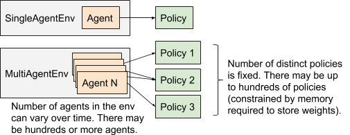
Figure 7: The multi-agent execution model in RLlib compared with single-agent execution.

Level 1: Multiple agents, shared policy

If all “agents” in the env are homogeneous (e.g., multiple independent cars in a traffic simulation), then it is possible to use existing single-agent algorithms for training. Since there is still only a single policy being trained, RLlib only needs to internally aggregate the experiences of the different agents prior to policy optimization. The change is minimal on the user side:

from single-agent:

register_env("your_env", lambda c: YourEnv(...))
trainer = PPOAgent(env="your_env")
while True:
    print(trainer.train())  # distributed training step

to multi-agent:

register_env("your_multi_env", lambda c: YourMultiEnv(...))
trainer = PPOAgent(env="your_multi_env")
while True:
    print(trainer.train())  # distributed training step

Note that the PPO “Agent” here is a just a naming convention carried over from the single-agent API. It acts more as a “trainer” of agents than an actual agent.

Level 2: Multiple agents, multiple policies

To handle multiple policies, this requires the definition of which agent(s) are handled by each policy. We handle this in RLlib via a policy mapping function, which assigns agents in the env to a particular policy when the agent first enters the environment. In the following examples we consider a hierarchical control setting where supervisor agents assign work to teams of worker agents they oversee. The desired configuration is to have a single supervisor policy and an ensemble of two worker policies:

def policy_mapper(agent_id):
    if agent_id.startswith("supervisor_"):
        return "supervisor_policy"
    else:
        return random.choice(["worker_p1", "worker_p2"])

In the example, we always bind supervisor agents to the single supervisor policy, and randomly divide other agents between an ensemble of two different worker policies. These assignments are done when the agent first enters the episode, and persist for the duration of the episode. Finally, we need to define the policy configurations, now that there is more than one. This is done as part of the top-level agent configuration:

trainer = PPOAgent(env="control_env", config={
    "multiagent": {
        "policy_mapping_fn": policy_mapper,
        "policy_graphs": {
            "supervisor_policy":
                (PPOPolicyGraph, sup_obs_space, sup_act_space, sup_conf),
            "worker_p1": (
                (PPOPolicyGraph, work_obs_s, work_act_s, work_p1_conf),
            "worker_p2":
                (PPOPolicyGraph, work_obs_s, work_act_s, work_p2_conf),
        },
        "policies_to_train": [
             "supervisor_policy", "worker_p1", "worker_p2"],
    },
})
while True:
    print(trainer.train())  # distributed training step

This would generate a configuration similar to that shown in Figure 2. You can pass in a custom policy graph class for each policy, as well as different policy config dicts. This allows for any of RLlib’s support for customization (e.g., custom models and preprocessors) to be used per policy, as well as wholesale definition of a new class of policy.

Advanced examples:

Level 3: Custom training strategies

For advanced applications or research use cases, it is inevitable to run into the limitations of any framework.

For example, let’s suppose multiple training methods are desired: some agents will learn with PPO, and others with DQN. This can be done in a way by swapping weights between two different trainers (there is a code example here), but this approach won’t scale with even more types of algorithms thrown in, or if e.g., you want to use experiences to train a model of the environment at the same time.

In these cases we can fall back to RLlib’s underlying system Ray to distribute computations as needed. Ray provides two simple parallel primitives:

Tasks, which are Python functions executed asynchronously via func.remote()
Actors, which are Python classes created in the cluster via class.remote(). Actor methods can be called via actor.method.remote().

RLlib builds on top of Ray tasks and actors to provide a toolkit for distributed RL training. This includes:

Policy graphs (as seen in previous examples)
Policy evaluation: the PolicyEvaluator class manages the environment interaction loop that generates batches of experiences. When created as Ray actors, it can be used to gather experiences in a distributed way.
Policy optimization: these implement distributed strategies for improving policies. You can use one of the existing optimizers or go with a custom strategy.

For example, you can create policy evaluators to gather multi-agent rollouts, and then process the batches as needed to improve the policies:

# Initialize a single-node Ray cluster
ray.init()

# Create local instances of your custom policy graphs
sup, w1, w2 = SupervisorPolicy(), WorkerPolicy(), WorkerPolicy()

# Create policy evaluators (Ray actor processes running in the cluster)
evaluators = []
for i in range(16):
    ev = PolicyEvaluator.as_remote().remote(
        env_creator=lambda ctx: ControlEnv(),
        policy_graph={
            "supervisor_policy": (SupervisorPolicy, ...),
            "worker_p1": ..., ...},
        policy_mapping_fn=policy_mapper,
        sample_batch_size=500)
    evaluators.append(ev)

while True:
    # Collect experiences in parallel using the policy evaluators
    futures = [ev.sample.remote() for ev in evaluators]
    batch = MultiAgentBatch.concat_samples(ray.get(futures))
    # >>> print(batch)
    # MultiAgentBatch({
    #     "supervisor_policy": SampleBatch({
    #          "obs": [[...], ...], "rewards": [0, ...], ...
    #      }),
    #     "worker_p1": SampleBatch(...),
    #     "worker_p2": SampleBatch(...),
    # })
    your_optimize_func(sup, w1, w2, batch)  # Custom policy optimization
    # Broadcast new weights and repeat
    for ev in evaluators:
        ev.set_weights.remote({
            "supervisor_policy": sup.get_weights(),
            "worker_p1": w1.get_weights(),
            "worker_p2": w2.get_weights(),
         })

In summary, RLlib provides several levels of APIs targeted at progressively more requirements for customizability. At the highest levels this provides a simple “out of the box” training process, but you retain the option to piece together your own algorithms and training strategies from the core multi-agent abstractions. To get started, here are a couple intermediate level scripts that can be run directly: multiagent_cartpole.py, multiagent_two_trainers.py.

Performance

RLlib is designed to scale to large clusters – and this applies to multi-agent mode as well – but we also apply optimizations such as vectorization for single-core efficiency. This allows for effective use of the multi-agent APIs on small machines.

To show the importance of these optimizations, in the below graph we plot single-core policy evaluation throughout vs the number of agents in the environment. For this benchmark the observations are small float vectors, and the policies are small 16x16 fully connected networks. We assign each agent to a random policy from a pool of 10 such policy networks. RLlib manages over 70k actions/s/core at 10000 agents per environment (the bottleneck becomes Python overhead at this point). When vectorization is turned off, experience collection slows down by 40x:

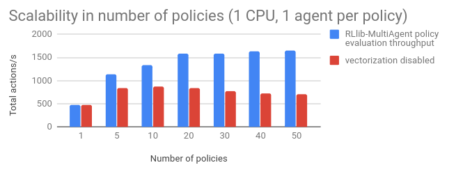
We also evaluate the more challenging case of having many distinct policy networks used in the environment. Here we can still leverage vectorization to fuse multiple TensorFlow calls into one, obtaining more stable per-core performance as the number of distinct policies scales from 1 to 50:

Conclusion

This blog post introduces a fast and general framework for multi-agent reinforcement learning. We’re currently working with early users of this framework in BAIR, the Berkeley Flow team, and industry to further improve RLlib. Try it out with 'pip install ray[rllib]' and tell us about your own use cases!

Documentation for RLlib and multi-agent support can be found at https://rllib.io.

Erin Grant, Eric Jang, and Eugene Vinitsky provided helpful input for this blog post.

Scaling Multi-Agent Reinforcement Learning