You’ve decided that you want to bike from your house by UC Berkeley to the Golden Gate Bridge. It’s a nice 20 mile ride, but there’s a problem: you’ve never ridden a bike before! To make matters worse, you are new to the Bay Area, and all you have is a good ol’ fashion map to guide you. How do you get started?
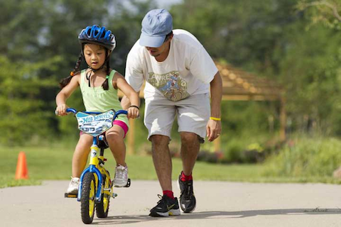
Let’s first figure out how to ride a bike. One strategy would be to do a lot of studying and planning. Read books on how to ride bicycles. Study physics and anatomy. Plan out all the different muscle movements that you’ll make in response to each perturbation. This approach is noble, but for anyone who’s ever learned to ride a bike, they know that this strategy is doomed to fail. There’s only one way to learn how to ride a bike: trial and error. Some tasks like riding a bike are just too complicated to plan out in your head.
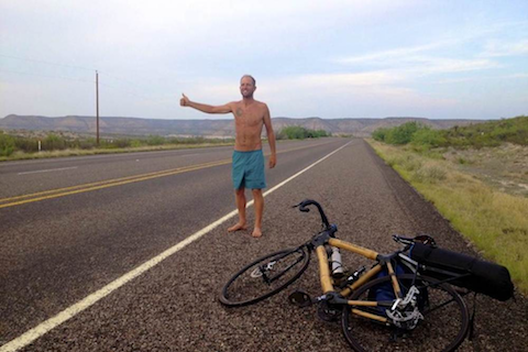
Once you’ve learned how to ride your bike, how would you get to the Golden Gate Bridge? You could reuse your trial-and-error strategy. Take a few random turns and see if you end up at the Golden Gate Bridge. Unfortunately, this strategy would take a very, very long time. For this sort of problem, planning is a much faster strategy, and requires considerably less real-world experience and trial-and-error. In reinforcement learning terms, it is more sample-efficient.
|
|
Left: some skills you learn by trial and error. Right: other times, planning ahead is better.
While simple, this thought experiment highlights some important aspects of human intelligence. For some tasks, we use a trial-and-error approach, and for others we use a planning approach. A similar phenomenon seems to have emerged in reinforcement learning (RL). In the parlance of RL, empirical results show that some tasks are better suited for model-free (trial-and-error) approaches, and others are better suited for model-based (planning) approaches.
However, the biking analogy also highlights that the two systems are not completely independent. In particularly, to say that learning to ride a bike is just trial-and-error is an oversimplification. In fact, when learning to bike by trial-and-error, you’ll employ a bit of planning. Perhaps your plan will initially be, “Don’t fall over.” As you improve, you’ll make more ambitious plans, such as, “Bike forwards for two meters without falling over.” Eventually, your bike-riding skills will be so proficient that you can start to plan in very abstract terms (“Bike to the end of the road.”) to the point that all there is left to do is planning and you no longer need to worry about the nitty-gritty details of riding a bike. We see that there is a gradual transition from the model-free (trial-and-error) strategy to a model-based (planning) strategy. If we could develop artificial intelligence algorithms--and specifically RL algorithms--that mimic this behavior, it could result in an algorithm that both performs well (by using trial-and-error methods early on) and is sample efficient (by later switching to a planning approach to achieve more abstract goals).
This post covers temporal difference model (TDM), which is a RL algorithm that captures this smooth transition between model-free and model-based RL. Before describing TDMs, we start by first describing how a typical model-based RL algorithm works.
Model-Based Reinforcement Learning
In reinforcement learning, we have some state space $\mathcal{S}$ and action space $\mathcal{A}$. If at time $t$ we are in state $s_t \in \mathcal{S}$ and take action $a_t\in \mathcal{A}$, we transition to a new state $s_{t+1} = f(s_t, a_t)$ according to a dynamics model $f: \mathcal{S} \times \mathcal{A} \mapsto \mathcal{S}$. The goal is to maximize rewards summed over the visited state: $\sum_{t=1}^{T-1} r(s_t, a_, s_{t+1})$. Model-based RL algorithms assume you are given (or learn) the dynamics model $f$. Given this dynamics model, there are a variety of model-based algorithms. For this post, we consider methods that perform the following optimization to choose a sequence of actions and states to maximize rewards:
The optimization says to choose a sequence of states and actions that you maximize the rewards, while ensuring that the trajectory is feasible. Here, feasible means that each state-action-next-state transition is valid. For example, in the image below if you start in state $s_t$ and take action $a_t$, only the top $s_{t+1}$ results in a feasible transition.

Planning a trip to the Golden Gate Bridge would be much easier if you could defy
physics. However, the constraint in the model-based optimization problem ensures
that only trajectories like the top row will be outputted. The bottom two
trajectories may have high reward, but they’re not feasible.
In our biking problem, the optimization might result in a biking plan from Berkeley (top right) to the Golden Gate Bridge (middle left) that looks like this:

An example of a plan (states and actions) outputted by solving the optimization problem.
While conceptually nice, this plan is not very realistic. Model-based approaches use a model $f(s, a)$ that predicts the state at the very next time step. In robotics, a time step usually corresponds to a tenth or a hundredth of a second. So perhaps a more realistic depiction of the resulting plan might look like:
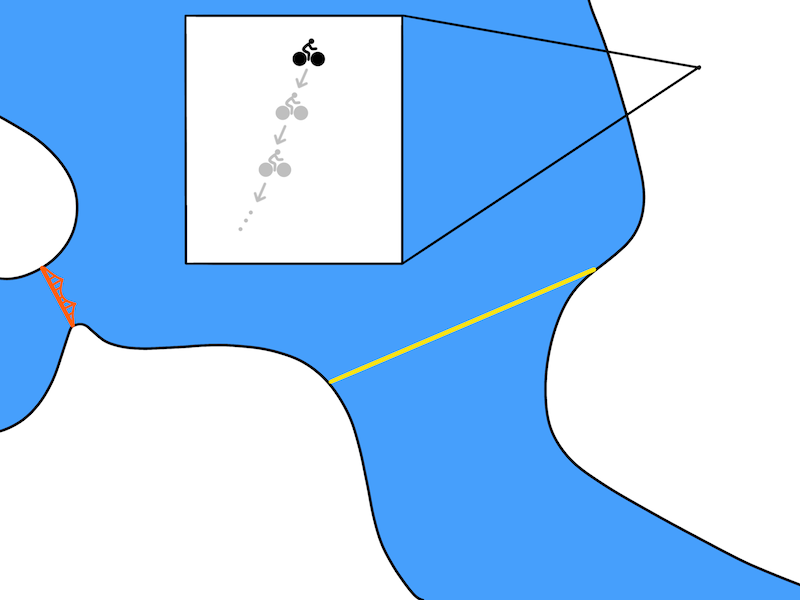
A more realistic plan.
If we think about how we plan in everyday life, we realize that we plan at much more temporally abstract terms. Rather than planning the position that our bike will be at the next tenth of a second, we make longer-term plans like, “I will go to the end of the road.” Furthermore, we can only make these temporally abstract plans once we’ve learned how to ride a bike in the first place. As discussed earlier, we need some way to (1) start the learning using a trial-and-error approach and (2) provide a mechanism to gradually increase the level of abstraction that we use to plan. For this, we introduce temporal difference models.
Temporal Difference Models
A temporal difference model (TDM)$^\dagger$, which we will write as $Q(s, a, s_g, \tau)$, is a function that, given a state $s \in \mathcal{S}$, action $a \in \mathcal{A}$, and goal state $s_g \in \mathcal{S}$, predicts how close an agent can get to the goal within $\tau$ time steps. Intuitively, a TDM answers the question, “If I try to bike to San Francisco in 30 minutes, how close will I get?” For robotics, a natural way to measure closeness is to use Euclidean distance.
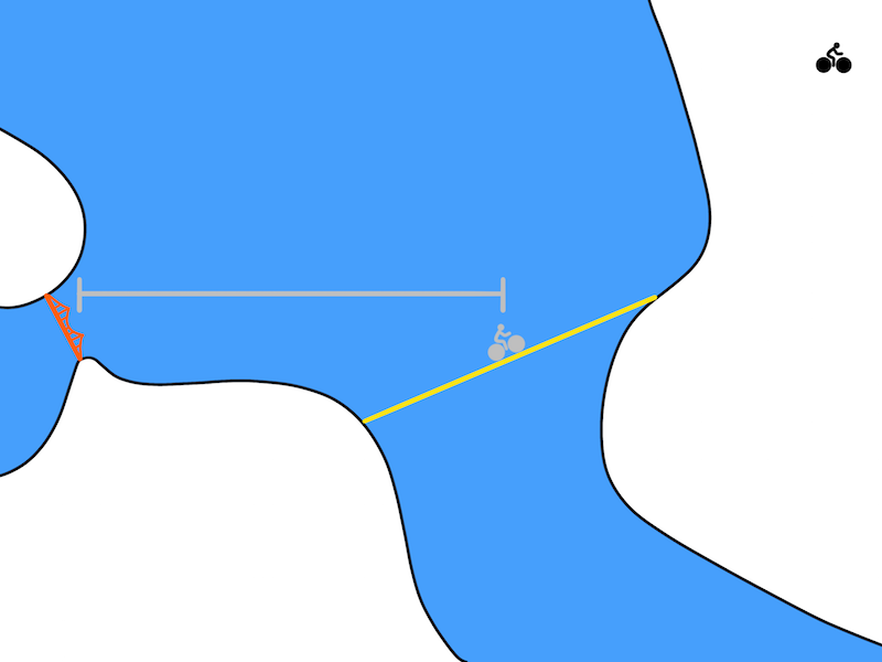
A TDM predicts how close you will get to the goal (Golden Gate Bridge) after a
fixed amount of time. After 30 minutes of biking, maybe you only reach the grey
biker in the image above. In this case, the grey line represents the distance
that the TDM should predict.
For those familiar with reinforcement learning, it turns out that a TDM can be viewed as a goal-conditioned Q function in a finite-horizon MDP. Because a TDM is just another Q function, we can train it with model-free (trial-and-error) algorithms. We use deep deterministic policy gradient (DDPG) to train a TDM and retroactively relabel the goal and time horizon to increase the sample efficiency of our learning algorithm. In theory, any Q-learning algorithm could be used to train the TDM, but we found this to be effective. We encourage readers to check out the paper for more details.
Planning with a TDM
Once we train a TDM, how can we use it to plan? It turns out that we can plan with the following optimization:
The intuition is similar to the model-based formulation. Choose a sequence of actions and states that maximize rewards and that are feasible. A key difference is that we only plan every $K$ time steps, rather than every time step. The constraint that $Q(s_t, a_t, s_{t+K}, K) = 0$ enforces the feasibility of the trajectory. Visually, rather than explicitly planning $K$ steps and actions like so

We can instead directly plan over $K$ time steps as shown below:

As we increase $K$, we get temporally more and more abstract plans. In between the $K$ time steps, we use a model-free approach to take actions, thereby allowing the model-free policy to “abstract away” the details of how the goal is actually reached. For the biking problem and for large enough values of $K$, the optimization could result in a plan like:

A model-based planner can be used to choose temporally abstract goals. A model-free algorithm can be used to reach those goals.
One caveat is that this formulation can only optimize the reward at every $K$ steps. However, many tasks only care about some states, such as the final state (e.g. “reach the Golden Gate Bridge”) and so this still captures a variety of interesting tasks.
Related Work
We’re not the first to look at the connection between model-based and model-free reinforcement. Parr ‘08 and Boyan ‘99, are particularly related, though they focus mainly on tabular and linear function approximators. The idea of training a goal condition Q function was also explored in Sutton ‘11 and Schaul ‘15, in the context of robot navigation and Atari games. Lastly, the relabelling scheme that we use is inspired by the work of Andrychowicz ‘17.
Experiments
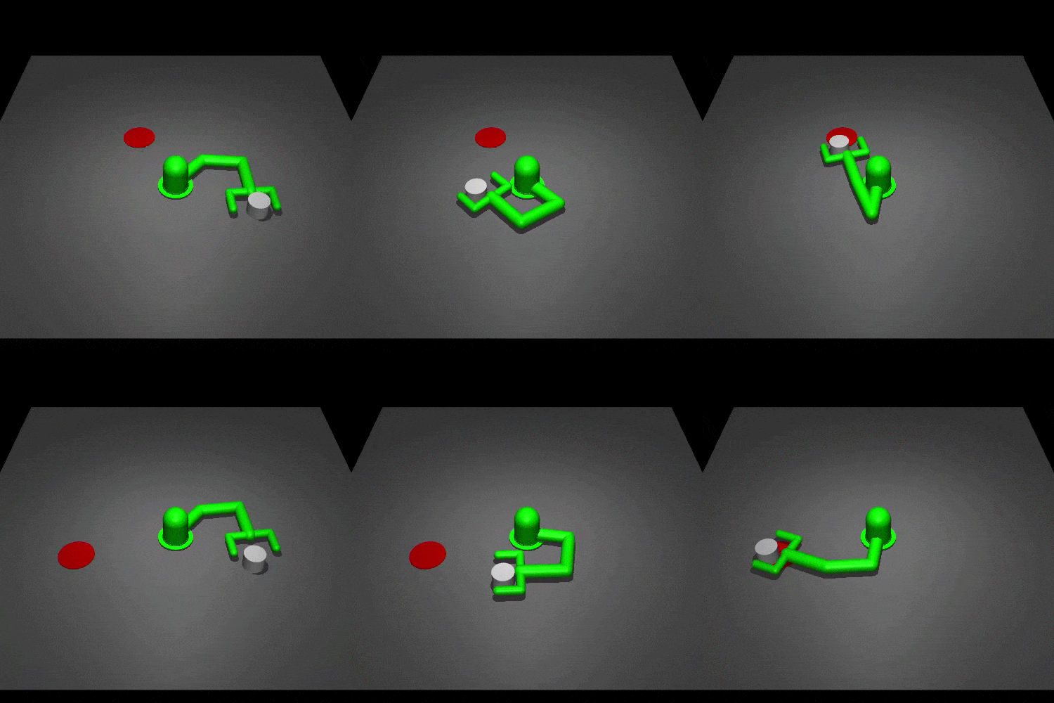
We tested TDMs on five simulated continuous control tasks and one real-world robotics task. One of the simulated tasks is to train a robot arm to push a cylinder to a target position. An example of the final pushing TDM policy and the associate learning curves are shown below:
|
|
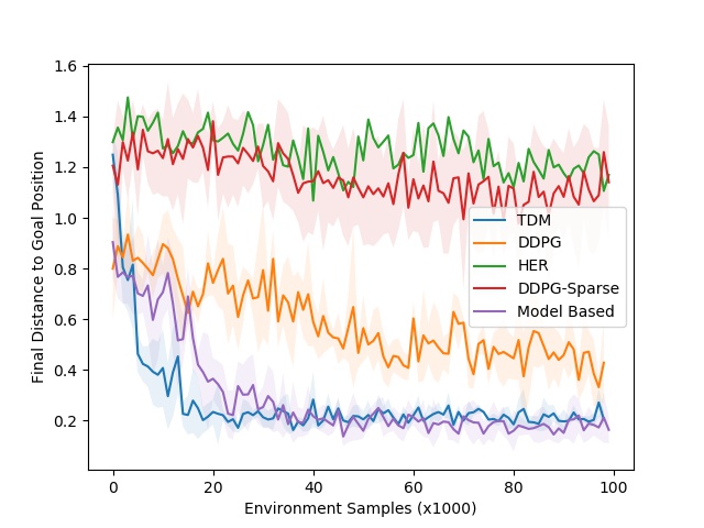
Left: TDM policy for reaching task. Right: Learning curves. TDM is blue (lower is better).
In the learning curve to the right, we plot the final distance to goal versus the number of environment samples (lower is better). Our simulation controls the robots at 20 Hz, meaning that 1000 steps corresponds to 50 seconds in the real world. The dynamics of this environment are relatively easy to learn, meaning that a model-based approach should excel. As expected, the model-based approaches (purple curve) learns quickly--roughly 3000 steps, or 25 minutes--and performs well. The TDM approach (blue curve) also learn quickly--roughly 2000 steps, or 17 minutes. The model-free DDPG (without TDMs) baseline eventually solves the task, but requires many more training samples. One reason the TDM approach learns so quickly is that it effectively is a model-based method in disguise.
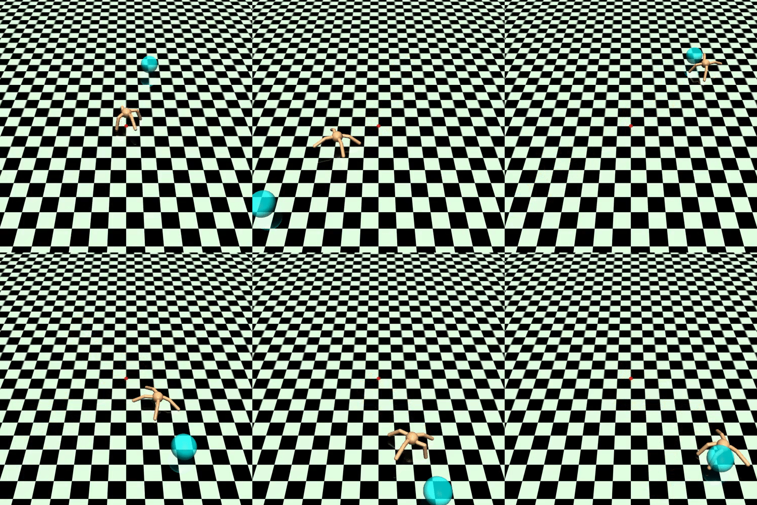
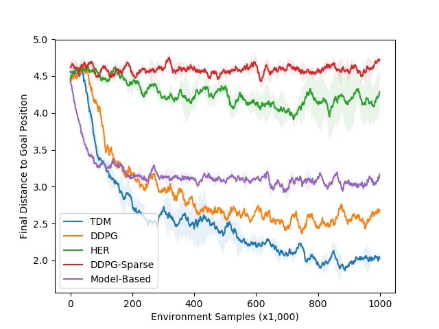
The story looks much better for model-free approaches when we move to locomotion tasks, which have substantially harder dynamics. One of the locomotion tasks involves training a quadruped robot to move to a certain position. The resulting TDM policy is shown below on the left, along with the accompanying learning curve on the right.
|
|
Left: TDM policy for locomotion task. Right: Learning curves. TDM is blue (lower is better).
Just as we use trial-and-error rather than planning to master riding a bicycle, we expect model-free methods to perform better than model-based methods on these locomotion tasks. This is precisely what we see in the learning curve on the right: the model-based method plateaus in performance. The model-free DDPG method learns more slowly, but eventually outperforms the model-based approach. TDM manages to both learn quickly and achieve good final performance. There are more experiments in the paper, including training a real-world 7 degree-of-freedom Sawyer to reach positions. We encourage the readers to check them out!
Future Directions
Temporal difference models provide a formalism and practical algorithm for interpolating from model-free to model-based control. However, there’s a lot of future work to be done. For one, the derivation assumes that the environment and policies are deterministic. In practice, most environments are stochastic. Even if they were deterministic, there are compelling reasons to use a stochastic policy in practice (see this blog post for one example). Extending TDMs to this setting would help move TDMs to more realistic environments. Another idea would be to combine TDMs with alternative model-based planning optimization algorithms than the ones we used in the paper. Lastly, we’d like to apply TDMs to more challenging tasks with real-world robots, like locomotion, manipulation, and, of course, bicycling to the Golden Gate Bridge.
This work will be presented at ICLR 2018. For more information about TDMs, check out the following links and come see us at our poster presentation at ICLR in Vancouver:
Let us know if you have any questions or comments!
$^\dagger$ We call it a temporal difference model because we train $Q$ with temporal difference learning and use $Q$ as a model.
I would like to thank Sergey Levine and Shane Gu for their valuable feedback when preparing this blog post.
