Feature selection is a common method for dimensionality reduction that encourages model interpretability. With large data sets becoming ever more prevalent, feature selection has seen widespread usage across a variety of real-world tasks in recent years, including text classification, gene selection from microarray data, and face recognition. We study the problem of supervised feature selection, which entails finding a subset of the input features that explains the output well. This practice can reduce the computational expense of downstream learning by removing features that are redundant or noisy, while simultaneously providing insight into the data through the features that remain.
Feature selection algorithms can generally be divided into three main categories: filter methods, wrapper methods, and embedded methods. Filter methods select features based on intrinsic properties of the data, independent of the learning algorithm to be used. For example, we may compute the correlation between each feature and the response variable, and select the variables with the highest correlation. Wrapper methods are more specialized in contrast, aiming to find features that optimize the performance of a specific predictor. For example, we may train multiple SVMs, each with a different subset of features, and choose the subset of features with the lowest loss on the training data. Because there are exponentially many subsets of features, wrapper methods often employ greedy algorithms. Finally, embedded methods are multipurpose techniques that incorporate feature selection and prediction into a single problem, often by optimizing an objective combining a goodness-of-fit term with a penalty on the number of parameters. One example is the LASSO method for constructing a linear model, which penalizes the coefficients with an $\ell_1$ penalty.
In this post, we propose conditional covariance minimization (CCM), a feature selection method that aims to unify the first two perspectives. We first describe our approach in the sections that follow. We then demonstrate through several synthetic experiments that our method is capable of capturing joint nonlinear relationships between collections of features. Finally, we show that our algorithm has performance comparable to or better than several other popular feature selection algorithms on a variety of real-world tasks.
Formulating feature selection
One way to view the problem of feature selection is from the lens of dependence. Ideally, we would like to identify a subset of features $\mathcal{T}$ of a pre-selected size $m$ such that the remaining features are conditionally independent of the responses given $\mathcal{T}$. However, this may not be achievable when $m$ is small. We therefore quantify the extent of the remaining conditional dependence using some metric, and aim to minimize it over all subsets $\mathcal{T}$ of the appropriate size.
Alternatively, we might like to find the subset of features $\mathcal{T}$ that can most effectively predict the output $Y$ within the context of a specific learning problem. The prediction error in our framework is defined as the mean square error between the labels and the predictions made by the best classifier selected from a class of functions.
Our method
We propose a criterion that can simultaneously characterize dependence and prediction error in regression. Roughly, we first introduce two function spaces on the domain of a subset of features $X_\mathcal{T}$ and the domain of the response variable $Y$ respectively. Each function space is a complete inner product space (Hilbert space) equipped with a kernel function which spans the whole space and has the ‘‘reproducing property’’. Such a function space is called a Reproducing Kernel Hilbert Space (RKHS). Then we define an operator for the RKHS over the domain of the response variable that characterizes the conditional dependence of the response variable on the input data given the selected features. Such an operator is called the conditional covariance operator. We use the trace of the operator computed with respect to the empirical distribution as our optimization criterion, which is also the estimated regression error of the best predictor within the given RKHS over the domain of the input data. Directly minimizing this criterion over subsets of features is computationally intractable. Instead, we formulate a relaxed problem by weighting each feature with a real-valued scalar between 0 and 1, and add an $\ell_1$-penalty over the weights. The objective of the relaxed problem can be represented in terms of kernel matrices, and is readily optimized using gradient-based approaches.
Results
We evaluate our approach on both synthetic and real-world data sets. We compare with several strong existing algorithms, including recursive feature elimination (RFE), Minimum Redundancy Maximum Relevance (mRMR), BAHSIC, and filter methods using mutual information (MI) and Pearson’s correlation (PC). RFE is a very popular wrapper method that greedily selects features based on the scores they receive from a classifier. mRMR selects features that capture different information from one another but each correlate well with the response variable. BAHSIC is a kernel method that greedily optimizes the dependence between selected features and the response variable. Lastly, filter methods employing MI or PC greedily optimize the respective metrics between selected subsets of features and the response.
Synthetic data
We use the following synthetic data sets:
-
Orange Skin. Given $Y=-1$, ten features $(X_1,\dots,X_{10})$ are independent standard normal random variables. Given $Y=1$, the first four features are standard normal random variables conditioned on $9 \leq \sum_{j=1}^4 X_j^2 \leq 16$, and the remaining six features $(X_5,\dots,X_{10})$ are independent standard normal random variables.
-
3-dimensional XOR as 4-way classification. Consider the 8 corners of the 3-dimensional hypercube $(v_1, v_2, v_3) \in \{-1,1\}^3$, and group them by the tuples $(v_1 v_3, v_2 v_3)$, leaving 4 sets of vectors paired with their negations $\{v^{(i)}, -v^{(i)}\}$. Given a class $i$, a sample is generated by selecting $v^{(i)}$ or $-v^{(i)}$ with equal probability and adding some noise. Each sample additionally has 7 standard normal noise features for a total of 10 dimensions.
-
Additive nonlinear regression. Consider the following additive model:
\[Y=-2\sin(2X_1)+\max(X_2,0)+X_3+\exp(-X_4)+\varepsilon.\]Each sample additionally has 6 noise features for a total of 10 dimensions. All features and the noise $\varepsilon$ are generated from standard normal distributions.
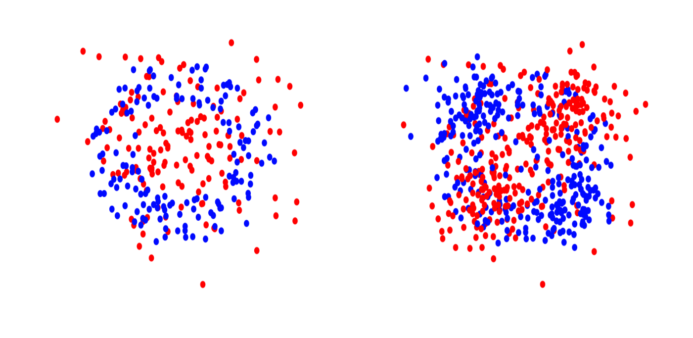
Left: Orange Skin in 2d. Right: XOR in 2d.
The first data set represents a standard nonlinear binary classification task. The second data set is a multi-class classification task where each feature is independent of $Y$ by itself but a combination of three features has a joint effect on $Y$. The third data set arises from an additive model for nonlinear regression.
Each data set has $d=10$ dimensions in total, but only $m=3$ or $4$ true features. Since the identity of these features is known, we can evaluate the performance of a given feature selection algorithm by computing the median rank it assigns to the real features, with lower median ranks indicating better performance.
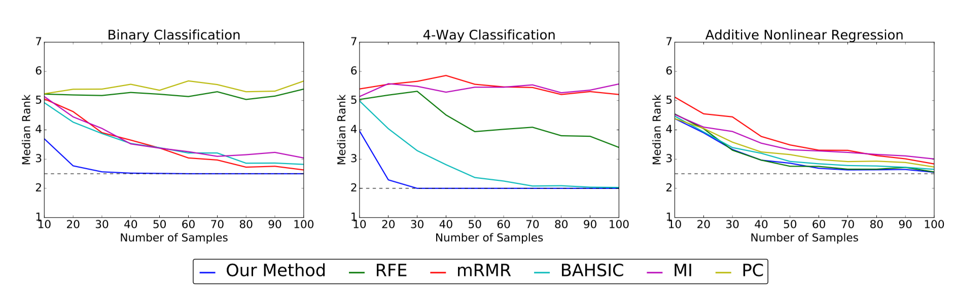
The above plots show the median rank (y-axis) of the true features as
a function of sample size (x-axis) for the simulated data sets. Lower median
ranks are better. The dotted line indicates the optimal median rank.
On the binary and 4-way classification tasks, our method outperforms all other algorithms, succeeding in identifying the true features using fewer than 50 samples where others require close to 100 or even fail to converge. On the additive nonlinear model, several algorithms perform well, and our method is on par with the best of them across all sample sizes.
Real-world data
We now turn our attention to a collection of real-word tasks, studying the performance of our method and other nonlinear approaches (mRMR, BAHSIC, MI) when used in conjunction with a kernel SVM for downstream classification.
We carry out experiments on 12 standard benchmark tasks from the ASU feature selection website and the UCI repository. A summary of our data sets is provided in the following table.
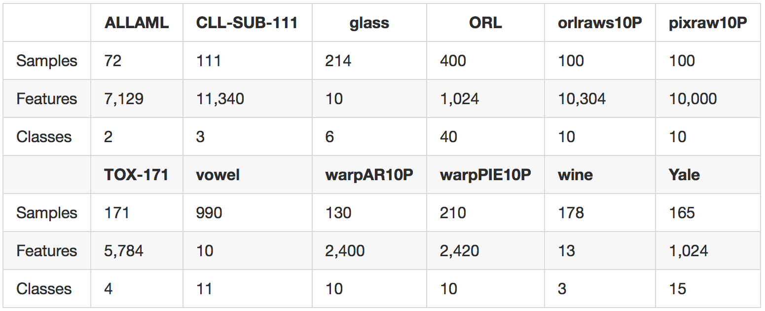
The data sets are drawn from several domains including gene data, image data, and voice data, and span both the low-dimensional and high-dimensional regimes.
For every task, we run each algorithm being evaluated to obtain ranks for all features. Performance is then measured by training a kernel SVM on the top $m$ features and computing the resulting accuracy. Our results are shown in the following figures.
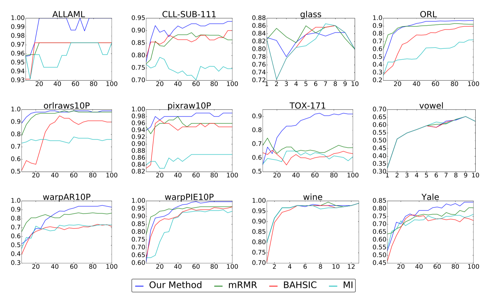
The above plots show classification accuracy (y-axis) versus number of
selected features (x-axis) for our real-world benchmark data sets. Higher
accuracies are better.
Compared with three other popular methods for nonlinear feature selection, we find that our method is the strongest performer in the large majority of cases, sometimes by a substantial margin as in the case of TOX-171. While our method is occasionally outperformed in the beginning when the number of selected features is small, it either ties or overtakes the leading method by the end in all but one instance.
Conclusion
In this post, we propose conditional covariance minimization (CCM), an approach to feature selection based on minimizing the trace of the conditional covariance operator. The idea is to select the features that maximally account for the dependence of the response on the covariates. We accomplish this by relaxing an intractable discrete formulation of the problem to obtain a continuous approximation suitable for gradient-based optimization. We demonstrate the effectiveness of our approach on multiple synthetic and real-world experiments, finding that it often outperforms other state-of-the-art approaches, including another competitive kernel feature selection method based on the Hilbert-Schmidt independence criterion.
More Information
For more information about our algorithm, please take a look at the following links:
Please let us know if you have any questions or suggestions.