Since we posted our paper on “Learning to Optimize” last year, the area of optimizer learning has received growing attention. In this article, we provide an introduction to this line of work and share our perspective on the opportunities and challenges in this area.

Machine learning has enjoyed tremendous success and is being applied to a wide variety of areas, both in AI and beyond. This success can be attributed to the data-driven philosophy that underpins machine learning, which favours automatic discovery of patterns from data over manual design of systems using expert knowledge.

Yet, there is a paradox in the current paradigm: the algorithms that power machine learning are still designed manually. This raises a natural question: can we learn these algorithms instead? This could open up exciting possibilities: we could find new algorithms that perform better than manually designed algorithms, which could in turn improve learning capability.

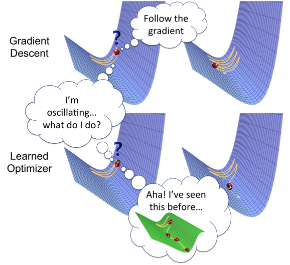
Doing so, however, requires overcoming a fundamental obstacle: how do we parameterize the space of algorithms so that it is both (1) expressive, and (2) efficiently searchable? Various ways of representing algorithms trade off these two goals. For example, if the space of algorithms is represented by a small set of known algorithms, it most likely does not contain the best possible algorithm, but does allow for efficient searching via simple enumeration of algorithms in the set. On the other hand, if the space of algorithms is represented by the set of all possible programs, it contains the best possible algorithm, but does not allow for efficient searching, as enumeration would take exponential time.

One of the most common types of algorithms used in machine learning is continuous optimization algorithms. Several popular algorithms exist, including gradient descent, momentum, AdaGrad and ADAM. We consider the problem of automatically designing such algorithms. Why do we want to do this? There are two reasons: first, many optimization algorithms are devised under the assumption of convexity and applied to non-convex objective functions; by learning the optimization algorithm under the same setting as it will actually be used in practice, the learned optimization algorithm could hopefully achieve better performance. Second, devising new optimization algorithms manually is usually laborious and can take months or years; learning the optimization algorithm could reduce the amount of manual labour.

Learning to Optimize

In our paper last year (Li & Malik, 2016), we introduced a framework for learning optimization algorithms, known as “Learning to Optimize”. We note that soon after our paper appeared, (Andrychowicz et al., 2016) also independently proposed a similar idea.

Consider how existing continuous optimization algorithms generally work. They operate in an iterative fashion and maintain some iterate, which is a point in the domain of the objective function. Initially, the iterate is some random point in the domain; in each iteration, a step vector is computed using some fixed update formula, which is then used to modify the iterate. The update formula is typically some function of the history of gradients of the objective function evaluated at the current and past iterates. For example, in gradient descent, the update formula is some scaled negative gradient; in momentum, the update formula is some scaled exponential moving average of the gradients.

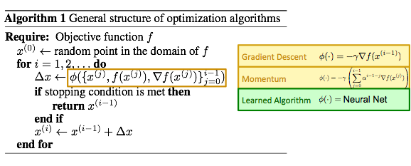
What changes from algorithm to algorithm is this update formula. So, if we can learn the update formula, we can learn an optimization algorithm. We model the update formula as a neural net. Thus, by learning the weights of the neural net, we can learn an optimization algorithm. Parameterizing the update formula as a neural net has two appealing properties mentioned earlier: first, it is expressive, as neural nets are universal function approximators and can in principle model any update formula with sufficient capacity; second, it allows for efficient search, as neural nets can be trained easily with backpropagation.

In order to learn the optimization algorithm, we need to define a performance metric, which we will refer to as the “meta-loss”, that rewards good optimizers and penalizes bad optimizers. Since a good optimizer converges quickly, a natural meta-loss would be the sum of objective values over all iterations (assuming the goal is to minimize the objective function), or equivalently, the cumulative regret. Intuitively, this corresponds to the area under the curve, which is larger when the optimizer converges slowly and smaller otherwise.

Learning to Learn

Consider the special case when the objective functions are loss functions for training other models. Under this setting, optimizer learning can be used for “learning to learn”. For clarity, we will refer to the model that is trained using the optimizer as the “base-model” and prefix common terms with “base-” and “meta-” to disambiguate concepts associated with the base-model and the optimizer respectively.

What do we mean exactly by “learning to learn”? While this term has appeared from time to time in the literature, different authors have used it to refer to different things, and there is no consensus on its precise definition. Often, it is also used interchangeably with the term “meta-learning”.

The term traces its origins to the idea of metacognition (Aristotle, 350 BC), which describes the phenomenon that humans not only reason, but also reason about their own process of reasoning. Work on “learning to learn” draws inspiration from this idea and aims to turn it into concrete algorithms. Roughly speaking, “learning to learn” simply means learning something about learning. What is learned at the meta-level differs across methods. We can divide various methods into three broad categories according to the type of meta-knowledge they aim to learn:

• Learning What to Learn
• Learning Which Model to Learn
• Learning How to Learn

Learning What to Learn

These methods aim to learn some particular values of base-model parameters that are useful across a family of related tasks (Thrun & Pratt, 2012). The meta-knowledge captures commonalities across the family, so that base-learning on a new task from the family can be done more quickly. Examples include methods for transfer learning, multi-task learning and few-shot learning. Early methods operate by partitioning the parameters of the base-model into two sets: those that are specific to a task and those that are common across tasks. For example, a popular approach for neural net base-models is to share the weights of the lower layers across all tasks, so that they capture the commonalities across tasks. See this post by Chelsea Finn for an overview of the more recent methods in this area.

Learning Which Model to Learn

These methods aim to learn which base-model is best suited for a task (Brazdil et al., 2008). The meta-knowledge captures correlations between different base-models and their performance on different tasks. The challenge lies in parameterizing the space of base-models in a way that is expressive and efficiently searchable, and in parameterizing the space of tasks that allows for generalization to unseen tasks. Different methods make different trade-offs between expressiveness and searchability: (Brazdil et al., 2003) uses a database of predefined base-models and exemplar tasks and outputs the base-model that performed the best on the nearest exemplar task. While this space of base-models is searchable, it does not contain good but yet-to-be-discovered base-models. (Schmidhuber, 2004) represents each base-model as a general-purpose program. While this space is very expressive, searching in this space takes exponential time in the length of the target program. (Hochreiter et al., 2001) views an algorithm that trains a base-model as a black box function that maps a sequence of training examples to a sequence of predictions and models it as a recurrent neural net. Meta-training then simply reduces to training the recurrent net. Because the base-model is encoded in the recurrent net’s memory state, its capacity is constrained by the memory size. A related area is hyperparameter optimization, which aims for a weaker goal and searches over base-models parameterized by a predefined set of hyperparameters. It needs to generalize across hyperparameter settings (and by extension, base-models), but not across tasks, since multiple trials with different hyperparameter settings on the same task are allowed.

Learning How to Learn

While methods in the previous categories aim to learn about the outcome of learning, methods in this category aim to learn about the process of learning. The meta-knowledge captures commonalities in the behaviours of learning algorithms. There are three components under this setting: the base-model, the base-algorithm for training the base-model, and the meta-algorithm that learns the base-algorithm. What is learned is not the base-model itself, but the base-algorithm, which trains the base-model on a task. Because both the base-model and the task are given by the user, the base-algorithm that is learned must work on a range of different base-models and tasks. Since most learning algorithms optimize some objective function, learning the base-algorithm in many cases reduces to learning an optimization algorithm. This problem of learning optimization algorithms was explored in (Li & Malik, 2016), (Andrychowicz et al., 2016) and a number of subsequent papers. Closely related to this line of work is (Bengio et al., 1991), which learns a Hebb-like synaptic learning rule. The learning rule depends on a subset of the dimensions of the current iterate encoding the activities of neighbouring neurons, but does not depend on the objective function and therefore does not have the capability to generalize to different objective functions.

Generalization

Learning of any sort requires training on a finite number of examples and generalizing to the broader class from which the examples are drawn. It is therefore instructive to consider what the examples and the class correspond to in our context of learning optimizers for training base-models. Each example is an objective function, which corresponds to the loss function for training a base-model on a task. The task is characterized by a set of examples and target predictions, or in other words, a dataset, that is used to train the base-model. The meta-training set consists of multiple objective functions and the meta-test set consists of different objective functions drawn from the same class. Objective functions can differ in two ways: they can correspond to different base-models, or different tasks. Therefore, generalization in this context means that the learned optimizer works on different base-models and/or different tasks.

Why is generalization important?

Suppose for moment that we didn’t care about generalization. In this case, we would evaluate the optimizer on the same objective functions that are used for training the optimizer. If we used only one objective function, then the best optimizer would be one that simply memorizes the optimum: this optimizer always converges to the optimum in one step regardless of initialization. In our context, the objective function corresponds to the loss for training a particular base-model on a particular task and so this optimizer essentially memorizes the optimal weights of the base-model. Even if we used many objective functions, the learned optimizer could still try to identify the objective function it is operating on and jump to the memorized optimum as soon as it does.

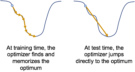
Why is this problematic? Memorizing the optima requires finding them in the first place, and so learning an optimizer takes longer than running a traditional optimizer like gradient descent. So, for the purposes of finding the optima of the objective functions at hand, running a traditional optimizer would be faster. Consequently, it would be pointless to learn the optimizer if we didn’t care about generalization.

Therefore, for the learned optimizer to have any practical utility, it must perform well on new objective functions that are different from those used for training.

What should be the extent of generalization?

If we only aim for generalization to similar base-models on similar tasks, then the learned optimizer could memorize parts of the optimal weights that are common across the base-models and tasks, like the weights of the lower layers in neural nets. This would be essentially the same as learning-what-to-learn formulations like transfer learning.

Unlike learning what to learn, the goal of learning how to learn is to learn not what the optimum is, but how to find it. We must therefore aim for a stronger notion of generalization, namely generalization to similar base-models on dissimilar tasks. An optimizer that can generalize to dissimilar tasks cannot just partially memorize the optimal weights, as the optimal weights for dissimilar tasks are likely completely different. For example, not even the lower layer weights in neural nets trained on MNIST(a dataset consisting of black-and-white images of handwritten digits) and CIFAR-10(a dataset consisting of colour images of common objects in natural scenes) likely have anything in common.

Should we aim for an even stronger form of generalization, that is, generalization to dissimilar base-models on dissimilar tasks? Since these correspond to objective functions that bear no similarity to objective functions used for training the optimizer, this is essentially asking if the learned optimizer should generalize to objective functions that could be arbitrarily different.

It turns out that this is impossible. Given any optimizer, we consider the trajectory followed by the optimizer on a particular objective function. Because the optimizer only relies on information at the previous iterates, we can modify the objective function at the last iterate to make it arbitrarily bad while maintaining the geometry of the objective function at all previous iterates. Then, on this modified objective function, the optimizer would follow the exact same trajectory as before and end up at a point with a bad objective value. Therefore, any optimizer has objective functions that it performs poorly on and no optimizer can generalize to all possible objective functions.

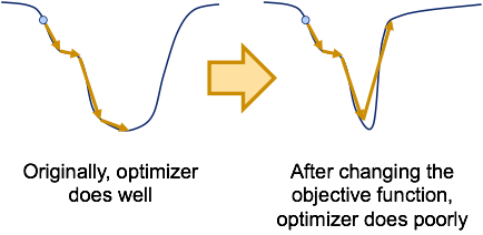
If no optimizer is universally good, can we still hope to learn optimizers that are useful? The answer is yes: since we are typically interested in optimizing functions from certain special classes in practice, it is possible to learn optimizers that work well on these classes of interest. The objective functions in a class can share regularities in their geometry, e.g.: they might have in common certain geometric properties like convexity, piecewise linearity, Lipschitz continuity or other unnamed properties. In the context of learning-how-to-learn, each class can correspond to a type of base-model. For example, neural nets with ReLU activation units can be one class, as they are all piecewise linear. Note that when learning the optimizer, there is no need to explicitly characterize the form of geometric regularity, as the optimizer can learn to exploit it automatically when trained on objective functions from the class.

How to Learn the Optimizer

The first approach we tried was to treat the problem of learning optimizers as a standard supervised learning problem: we simply differentiate the meta-loss with respect to the parameters of the update formula and learn these parameters using standard gradient-based optimization. (We weren’t the only ones to have thought of this; (Andrychowicz et al., 2016) also used a similar approach.)

This seemed like a natural approach, but it did not work: despite our best efforts, we could not get any optimizer trained in this manner to generalize to unseen objective functions, even though they were drawn from the same distribution that generated the objective functions used to train the optimizer. On almost all unseen objective functions, the learned optimizer started off reasonably, but quickly diverged after a while. On the other hand, on the training objective functions, it exhibited no such issues and did quite well. Why is this?

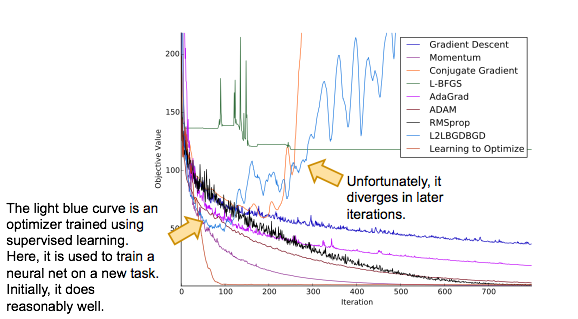
It turns out that optimizer learning is not as simple a learning problem as it appears. Standard supervised learning assumes all training examples are independent and identically distributed (i.i.d.); in our setting, the step vector the optimizer takes at any iteration affects the gradients it sees at all subsequent iterations. Furthermore, how the step vector affects the gradient at the subsequent iteration is not known, since this depends on the local geometry of the objective function, which is unknown at meta-test time. Supervised learning cannot operate in this setting, and must assume that the local geometry of an unseen objective function is the same as the local geometry of training objective functions at all iterations.

Consider what happens when an optimizer trained using supervised learning is used on an unseen objective function. It takes a step, and discovers at the next iteration that the gradient is different from what it expected. It then recalls what it did on the training objective functions when it encountered such a gradient, which could have happened in a completely different region of the space, and takes a step accordingly. To its dismay, it finds out that the gradient at the next iteration is even more different from what it expected. This cycle repeats and the error the optimizer makes becomes bigger and bigger over time, leading to rapid divergence.

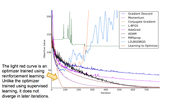
This phenomenon is known in the literature as the problem of compounding errors. It is known that the total error of a supervised learner scales quadratically in the number of iterations, rather than linearly as would be the case in the i.i.d. setting (Ross and Bagnell, 2010). In essence, an optimizer trained using supervised learning necessarily overfits to the geometry of the training objective functions. One way to solve this problem is to use reinforcement learning.

Background on Reinforcement Learning

Consider an environment that maintains a state, which evolves in an unknown fashion based on the action that is taken. We have an agent that interacts with this environment, which sequentially selects actions and receives feedback after each action is taken on how good or bad the new state is. The goal of reinforcement learning is to find a way for the agent to pick actions based on the current state that leads to good states on average.

More precisely, a reinforcement learning problem is characterized by the following components:

• A state space, which is the set of all possible states,
• An action space, which is the set of all possible actions,
• A cost function, which measures how bad a state is,
• A time horizon, which is the number of time steps,
• An initial state probability distribution, which specifies how frequently different states occur at the beginning before any action is taken, and
• A state transition probability distribution, which specifies how the state changes (probabilistically) after a particular action is taken.

While the learning algorithm is aware of what the first five components are, it does not know the last component, i.e.: how states evolve based on actions that are chosen. At training time, the learning algorithm is allowed to interact with the environment. Specifically, at each time step, it can choose an action to take based on the current state. Then, based on the action that is selected and the current state, the environment samples a new state, which is observed by the learning algorithm at the subsequent time step. The sequence of sampled states and actions is known as a trajectory. This sampling procedure induces a distribution over trajectories, which depends on the initial state and transition probability distributions and the way action is selected based on the current state, the latter of which is known as a policy. This policy is often modelled as a neural net that takes in the current state as input and outputs the action. The goal of the learning algorithm is to find a policy such that the expected cumulative cost of states over all time steps is minimized, where the expectation is taken with respect to the distribution over trajectories.

Formulation as a Reinforcement Learning Problem

Recall the learning framework we introduced above, where the goal is to find the update formula that minimizes the meta-loss. Intuitively, we think of the agent as an optimization algorithm and the environment as being characterized by the family of objective functions that we’d like to learn an optimizer for. The state consists of the current iterate and some features along the optimization trajectory so far, which could be some statistic of the history of gradients, iterates and objective values. The action is the step vector that is used to update the iterate.

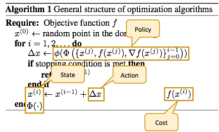
Under this formulation, the policy is essentially a procedure that computes the action, which is the step vector, from the state, which depends on the current iterate and the history of gradients, iterates and objective values. In other words, a particular policy represents a particular update formula. Hence, learning the policy is equivalent to learning the update formula, and hence the optimization algorithm. The initial state probability distribution is the joint distribution of the initial iterate, gradient and objective value. The state transition probability distribution characterizes what the next state is likely to be given the current state and action. Since the state contains the gradient and objective value, the state transition probability distribution captures how the gradient and objective value are likely to change for any given step vector. In other words, it encodes the likely local geometries of the objective functions of interest. Crucially, the reinforcement learning algorithm does not have direct access to this state transition probability distribution, and therefore the policy it learns avoids overfitting to the geometry of the training objective functions.

We choose a cost function of a state to be the value of the objective function evaluated at the current iterate. Because reinforcement learning minimizes the cumulative cost over all time steps, it essentially minimizes the sum of objective values over all iterations, which is the same as the meta-loss.

Results

We trained an optimization algorithm on the problem of training a neural net on MNIST, and tested it on the problems of training different neural nets on the Toronto Faces Dataset (TFD), CIFAR-10 and CIFAR-100. These datasets bear little similarity to each other: MNIST consists of black-and-white images of handwritten digits, TFD consists of grayscale images of human faces, and CIFAR-10/100 consists of colour images of common objects in natural scenes. It is therefore unlikely that a learned optimization algorithm can get away with memorizing, say, the lower layer weights, on MNIST and still do well on TFD and CIFAR-10/100.

As shown, the optimization algorithm trained using our approach on MNIST (shown in light red) generalizes to TFD, CIFAR-10 and CIFAR-100 and outperforms other optimization algorithms.

To understand the behaviour of optimization algorithms learned using our approach, we trained an optimization algorithm on two-dimensional logistic regression problems and visualized its trajectory in the space of the parameters. It is worth noting that the behaviours of optimization algorithms in low dimensions and high dimensions may be different, and so the visualizations below may not be indicative of the behaviours of optimization algorithms in high dimensions. However, they provide some useful intuitions about the kinds of behaviour that can be learned.

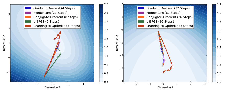
The plots above show the optimization trajectories followed by various algorithms on two different unseen logistic regression problems. Each arrow represents one iteration of an optimization algorithm. As shown, the algorithm learned using our approach (shown in light red) takes much larger steps compared to other algorithms. In the first example, because the learned algorithm takes large steps, it overshoots after two iterations, but does not oscillate and instead takes smaller steps to recover. In the second example, due to vanishing gradients, traditional optimization algorithms take small steps and therefore converge slowly. On the other hand, the learned algorithm takes much larger steps and converges faster.

Papers

More details can be found in our papers:

Learning to Optimize
Ke Li, Jitendra Malik
arXiv:1606.01885, 2016 and International Conference on Learning Representations (ICLR), 2017

Learning to Optimize Neural Nets
Ke Li, Jitendra Malik
arXiv:1703.00441, 2017

I’d like to thank Jitendra Malik for his valuable feedback.